PyTorch線性回歸

在本章中，我們將重點介紹使用TensorFlow進行線性回歸實現的基本範例。邏輯回歸或線性回歸是用於對離散類別進行分類的監督機器學習方法。在本章中的目標是構建一個模型，使用者可以通過該模型預測預測變數與一個或多個自變數之間的關係。

如果y是因變數x而變化，則x認為是自變數。兩個變數之間的這種關係可認為是線性的。兩個變數的線性回歸關係看起來就像下面提到的方程式一樣 -

Y = Ax+b

接下來，我們將設計一個線性回歸演算法，有助於理解下面給出的兩個重要概念 -

• 成本函式
• 梯度下降演算法

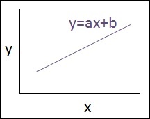
下面提到線性回歸的示意圖，解釋結果 -

Y=ax+b

• a的值是斜率。
• b的值是y -截距。
• r是相關係數。
• r^2是相關係數。

線性回歸方程的圖形檢視如下所述 -

以下步驟用於使用PyTorch實現線性回歸 -

第1步

使用以下程式碼匯入在PyTorch中建立線性回歸所需的包 -

import numpy as np
import matplotlib.pyplot as plt
from matplotlib.animation import FuncAnimation
import seaborn as sns
import pandas as pd
%matplotlib inline

sns.set_style(style = 'whitegrid')
plt.rcParams["patch.force_edgecolor"] = True

第2步

使用可用資料集建立單個訓練集，如下所示 -

m = 2 # slope
c = 3 # interceptm = 2 # slope
c = 3 # intercept
x = np.random.rand(256)

noise = np.random.randn(256) / 4

y = x * m + c + noise

df = pd.DataFrame()
df['x'] = x
df['y'] = y

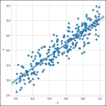
sns.lmplot(x ='x', y ='y', data = df)

得到的結果如下所示：

第3步

使用PyTorch庫實現線性回歸，如下所述 -

import torch
import torch.nn as nn
from torch.autograd import Variable
x_train = x.reshape(-1, 1).astype('float32')
y_train = y.reshape(-1, 1).astype('float32')

class LinearRegressionModel(nn.Module):
   def __init__(self, input_dim, output_dim):
      super(LinearRegressionModel, self).__init__()
      self.linear = nn.Linear(input_dim, output_dim)

   def forward(self, x):
      out = self.linear(x)
      return out
input_dim = x_train.shape[1]
output_dim = y_train.shape[1]
input_dim, output_dim(1, 1)
model = LinearRegressionModel(input_dim, output_dim)
criterion = nn.MSELoss()
[w, b] = model.parameters()

def get_param_values():
   return w.data[0][0], b.data[0]

def plot_current_fit(title = ""):
plt.figure(figsize = (12,4))
plt.title(title)
plt.scatter(x, y, s = 8)
w1 = w.data[0][0]
b1 = b.data[0]
x1 = np.array([0., 1.])
y1 = x1 * w1 + b1
plt.plot(x1, y1, 'r', label = 'Current Fit ({:.3f}, {:.3f})'.format(w1, b1))
plt.xlabel('x (input)')
plt.ylabel('y (target)')
plt.legend()
plt.show()
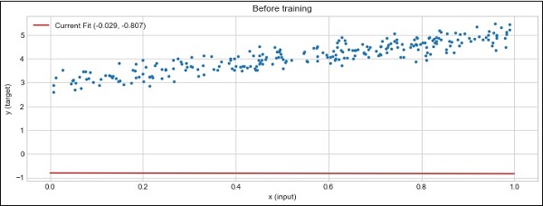
plot_current_fit('Before training')

執行上面範例程式碼，得到以下結果 -