Python----數據分析-使用scikit-learn構建模型
Python----數據分析-使用scikit-learn構建模型
scikit-learn庫整合了許多機器學習演算法,可以幫助使用者在數據分析過程中快速建立模型,且模型介面統一,使用起來很方便。
官網入口:https://scikit-learn.org/stable/modules/classes.html
目錄:
一、使用sklearn轉換器處理
1.載入datasets中的數據集
2.劃分數據集:訓練集、測試集
3.使用sklearn轉換器進行數據預處理與降維
二、構建評價聚類模型
1.使用sklearn估計器構建聚類模型
2.評價聚類模型
三、構建評價分類模型
1.使用sklearn估計器構建分類模型
2.評價分類模型
四、構建評價迴歸模型
1.使用sklearn估計器構建迴歸模型
2.評價迴歸模型
一、使用sklearn轉換器處理
sklearn提供了model_selection模型選擇模組、preprocessing數據預處理模組、decompisition特徵分解模組,通過這三個模組能夠實現數據的預處理和模型構建前的數據標準化、二值化、數據集的分割、交叉驗證和PCA降維處理等工作。
1.載入datasets中的數據集
sklearn庫的datasets模組整合了部分數據分析的經典數據集,可以選用進行數據預處理、建模的操作。
常見的數據集載入函數(器)
| 數據集載入函數(器) | 數據集任務型別 |
|---|---|
| load_digits | 分類 |
| load_wine | 分類 |
| load_iris | 分類、聚類 |
| load_breast_cancer | 分類、聚類 |
| load_boston | 迴歸 |
| fetch_california_housing | 迴歸 |
載入後的數據集可以看成是一個字典,幾乎所有的sklearn數據集均可以使用data、target、feature_names、DESCR分別獲取數據集的數據、標籤、特徵名稱、描述資訊。
以load_breast_cancer爲例:
from sklearn.datasets import load_breast_cancer

cancer = load_breast_cancer()##將數據集賦值給iris變數

print('breast_cancer數據集的長度爲:',len(cancer))
print('breast_cancer數據集的型別爲:',type(cancer))
#breast_cancer數據集的長度爲: 6
#breast_cancer數據集的型別爲: <class 'sklearn.utils.Bunch'>

cancer_data = cancer['data']
print('breast_cancer數據集的數據爲:','\n',cancer_data)
#breast_cancer數據集的數據爲:
 [[1.799e+01 1.038e+01 1.228e+02 ... 2.654e-01 4.601e-01 1.189e-01]
 [2.057e+01 1.777e+01 1.329e+02 ... 1.860e-01 2.750e-01 8.902e-02]
 [1.969e+01 2.125e+01 1.300e+02 ... 2.430e-01 3.613e-01 8.758e-02]
 ...
 [1.660e+01 2.808e+01 1.083e+02 ... 1.418e-01 2.218e-01 7.820e-02]
 [2.060e+01 2.933e+01 1.401e+02 ... 2.650e-01 4.087e-01 1.240e-01]
 [7.760e+00 2.454e+01 4.792e+01 ... 0.000e+00 2.871e-01 7.039e-02]]

cancer_target = cancer['target'] ## 取出數據集的標籤
print('breast_cancer數據集的標籤爲:\n',cancer_target)
#breast_cancer數據集的標籤爲:
 [0 0 0 0 0 0 0 0 0 0 0 0 0 0 0 0 0 0 0 1 1 1 0 0 0 0 0 0 0 0 0 0 0 0 0 0 0
 1 0 0 0 0 0 0 0 0 1 0 1 1 1 1 1 0 0 1 0 0 1 1 1 1 0 1 0 0 1 1 1 1 0 1 0 0
 1 0 1 0 0 1 1 1 0 0 1 0 0 0 1 1 1 0 1 1 0 0 1 1 1 0 0 1 1 1 1 0 1 1 0 1 1
 1 1 1 1 1 1 0 0 0 1 0 0 1 1 1 0 0 1 0 1 0 0 1 0 0 1 1 0 1 1 0 1 1 1 1 0 1
 1 1 1 1 1 1 1 1 0 1 1 1 1 0 0 1 0 1 1 0 0 1 1 0 0 1 1 1 1 0 1 1 0 0 0 1 0
 1 0 1 1 1 0 1 1 0 0 1 0 0 0 0 1 0 0 0 1 0 1 0 1 1 0 1 0 0 0 0 1 1 0 0 1 1
 1 0 1 1 1 1 1 0 0 1 1 0 1 1 0 0 1 0 1 1 1 1 0 1 1 1 1 1 0 1 0 0 0 0 0 0 0
 0 0 0 0 0 0 0 1 1 1 1 1 1 0 1 0 1 1 0 1 1 0 1 0 0 1 1 1 1 1 1 1 1 1 1 1 1
 1 0 1 1 0 1 0 1 1 1 1 1 1 1 1 1 1 1 1 1 1 0 1 1 1 0 1 0 1 1 1 1 0 0 0 1 1
 1 1 0 1 0 1 0 1 1 1 0 1 1 1 1 1 1 1 0 0 0 1 1 1 1 1 1 1 1 1 1 1 0 0 1 0 0
 0 1 0 0 1 1 1 1 1 0 1 1 1 1 1 0 1 1 1 0 1 1 0 0 1 1 1 1 1 1 0 1 1 1 1 1 1
 1 0 1 1 1 1 1 0 1 1 0 1 1 1 1 1 1 1 1 1 1 1 1 0 1 0 0 1 0 1 1 1 1 1 0 1 1
 0 1 0 1 1 0 1 0 1 1 1 1 1 1 1 1 0 0 1 1 1 1 1 1 0 1 1 1 1 1 1 1 1 1 1 0 1
 1 1 1 1 1 1 0 1 0 1 1 0 1 1 1 1 1 0 0 1 0 1 0 1 1 1 1 1 0 1 1 0 1 0 1 0 0
 1 1 1 0 1 1 1 1 1 1 1 1 1 1 1 0 1 0 0 1 1 1 1 1 1 1 1 1 1 1 1 1 1 1 1 1 1
 1 1 1 1 1 1 1 0 0 0 0 0 0 1]

cancer_names = cancer['feature_names'] ## 取出數據集的特徵名
print('breast_cancer數據集的特徵名爲:\n',cancer_names)
#breast_cancer數據集的特徵名爲:
 ['mean radius' 'mean texture' 'mean perimeter' 'mean area'
 'mean smoothness' 'mean compactness' 'mean concavity'
 'mean concave points' 'mean symmetry' 'mean fractal dimension'
 'radius error' 'texture error' 'perimeter error' 'area error'
 'smoothness error' 'compactness error' 'concavity error'
 'concave points error' 'symmetry error' 'fractal dimension error'
 'worst radius' 'worst texture' 'worst perimeter' 'worst area'
 'worst smoothness' 'worst compactness' 'worst concavity'
 'worst concave points' 'worst symmetry' 'worst fractal dimension']

cancer_desc = cancer['DESCR'] ## 取出數據集的描述資訊
print('breast_cancer數據集的描述資訊爲:\n',cancer_desc)
#breast_cancer數據集的描述資訊爲:
 .. _breast_cancer_dataset:

Breast cancer wisconsin (diagnostic) dataset
--------------------------------------------

**Data Set Characteristics:**

    :Number of Instances: 569

    :Number of Attributes: 30 numeric, predictive attributes and the class

    :Attribute Information:
        - radius (mean of distances from center to points on the perimeter)
        - texture (standard deviation of gray-scale values)
        - perimeter
        - area
        - smoothness (local variation in radius lengths)
        - compactness (perimeter^2 / area - 1.0)
        - concavity (severity of concave portions of the contour)
        - concave points (number of concave portions of the contour)
        - symmetry
        - fractal dimension ("coastline approximation" - 1)

        The mean, standard error, and "worst" or largest (mean of the three
        largest values) of these features were computed for each image,
        resulting in 30 features.  For instance, field 3 is Mean Radius, field
        13 is Radius SE, field 23 is Worst Radius.

        - class:
                - WDBC-Malignant
                - WDBC-Benign

    :Summary Statistics:

    ===================================== ====== ======
                                           Min    Max
    ===================================== ====== ======
    radius (mean):                        6.981  28.11
    texture (mean):                       9.71   39.28
    perimeter (mean):                     43.79  188.5
    area (mean):                          143.5  2501.0
    smoothness (mean):                    0.053  0.163
    compactness (mean):                   0.019  0.345
    concavity (mean):                     0.0    0.427
    concave points (mean):                0.0    0.201
    symmetry (mean):                      0.106  0.304
    fractal dimension (mean):             0.05   0.097
    radius (standard error):              0.112  2.873
    texture (standard error):             0.36   4.885
    perimeter (standard error):           0.757  21.98
    area (standard error):                6.802  542.2
    smoothness (standard error):          0.002  0.031
    compactness (standard error):         0.002  0.135
    concavity (standard error):           0.0    0.396
    concave points (standard error):      0.0    0.053
    symmetry (standard error):            0.008  0.079
    fractal dimension (standard error):   0.001  0.03
    radius (worst):                       7.93   36.04
    texture (worst):                      12.02  49.54
    perimeter (worst):                    50.41  251.2
    area (worst):                         185.2  4254.0
    smoothness (worst):                   0.071  0.223
    compactness (worst):                  0.027  1.058
    concavity (worst):                    0.0    1.252
    concave points (worst):               0.0    0.291
    symmetry (worst):                     0.156  0.664
    fractal dimension (worst):            0.055  0.208
    ===================================== ====== ======

    :Missing Attribute Values: None

    :Class Distribution: 212 - Malignant, 357 - Benign

    :Creator:  Dr. William H. Wolberg, W. Nick Street, Olvi L. Mangasarian

    :Donor: Nick Street

    :Date: November, 1995

This is a copy of UCI ML Breast Cancer Wisconsin (Diagnostic) datasets.
https://goo.gl/U2Uwz2

Features are computed from a digitized image of a fine needle
aspirate (FNA) of a breast mass.  They describe
characteristics of the cell nuclei present in the image.

Separating plane described above was obtained using
Multisurface Method-Tree (MSM-T) [K. P. Bennett, "Decision Tree
Construction Via Linear Programming." Proceedings of the 4th
Midwest Artificial Intelligence and Cognitive Science Society,
pp. 97-101, 1992], a classification method which uses linear
programming to construct a decision tree.  Relevant features
were selected using an exhaustive search in the space of 1-4
features and 1-3 separating planes.

The actual linear program used to obtain the separating plane
in the 3-dimensional space is that described in:
[K. P. Bennett and O. L. Mangasarian: "Robust Linear
Programming Discrimination of Two Linearly Inseparable Sets",
Optimization Methods and Software 1, 1992, 23-34].

This database is also available through the UW CS ftp server:

ftp ftp.cs.wisc.edu
cd math-prog/cpo-dataset/machine-learn/WDBC/

.. topic:: References

   - W.N. Street, W.H. Wolberg and O.L. Mangasarian. Nuclear feature extraction
     for breast tumor diagnosis. IS&T/SPIE 1993 International Symposium on
     Electronic Imaging: Science and Technology, volume 1905, pages 861-870,
     San Jose, CA, 1993.
   - O.L. Mangasarian, W.N. Street and W.H. Wolberg. Breast cancer diagnosis and
     prognosis via linear programming. Operations Research, 43(4), pages 570-577,
     July-August 1995.
   - W.H. Wolberg, W.N. Street, and O.L. Mangasarian. Machine learning techniques
     to diagnose breast cancer from fine-needle aspirates. Cancer Letters 77 (1994)
     163-171.
2.劃分數據集:訓練集、測試集
在數據分析的過程中,爲了保證模型在實際系統中能夠起到預期的作用,一般需要將樣本分成獨立的三部分:訓練集(train set)、驗證集(validation set)、測試集(test set)。
訓練集—50%:用於估計模型
驗證集—25%:用於確定網路結構或控制模型複雜程度的參數
測試集—25%:用於檢驗最優模型的效能
當數據總量較少的時候,使用上述方法劃分就不合適。常用的方法是留少部分做測試集,然後對其餘N個樣本採用K折交叉驗證法:
將樣本打亂,並均勻分成K份,輪流選擇其中K-1份做訓練,剩餘一份做檢驗,計算預測誤差平方和,最後把K次的預測誤差平方和的均值作爲選擇最優模型結構的依據。
sklearn.model_selection.train_test_split(*arrays,**options)
| 參數名稱 | 說明 |
|---|---|
| *arrays | 接受一個或者多個數據集。代表需要劃分的數據集。若爲分類、迴歸,則傳入數據、標籤;若爲聚類,則傳入數據 |
| test_size | 代表測試集的大小。若傳入爲float型別數據,需要限定在0-1之間,代表測試集在總數中的佔比;若傳入的爲int型數據,則表示測試集記錄的絕對數目。該參數與train_size可以只傳入一個。 |
| train_size | 與test_size相同 |
| random_state | 接受int。代表隨機種子編號,相同隨機種子編號產生相同的隨機結果。 |
| shuffle | 接受boolean。代表是否進行有回放抽樣,若爲True,則stratify參數必須不能爲空。 |
| stratify | 接受array或None。若不爲None,則使用傳入的標籤進行分層抽樣。 |
print('原始數據集數據的形狀爲:',cancer_data.shape)
print('原始數據集標籤的形狀爲:',cancer_target.shape)
原始數據集數據的形狀爲: (569, 30)
原始數據集標籤的形狀爲: (569,)

from sklearn.model_selection import train_test_split

cancer_data_train,cancer_data_test,cancer_target_train,cancer_target_test = train_test_split(cancer_data,cancer_target,
                                                                                             test_size=0.2,random_state=42)
print('訓練集數據的形狀爲:',cancer_data_train.shape)
print('訓練集數據的標籤形狀爲:',cancer_target_train.shape)
print('測試集數據的形狀爲:',cancer_data_test.shape)
print('測試集數據的標籤形狀爲:',cancer_target_test.shape)
訓練集數據的形狀爲: (455, 30)
訓練集數據的標籤形狀爲: (455,)
測試集數據的形狀爲: (114, 30)
測試集數據的標籤形狀爲: (114,)
該函數分別將傳入的數據劃分爲訓練集和測試集。如果傳入的是一組數據,那麼生成的就是這一組數據隨機劃分後的訓練集和測試集,總共兩組;如果傳入的是兩組數據,那麼生成的訓練集和測試集分別兩組,總共四組。
train_test_split方法僅是最常用的數據劃分方法,在model_selection模組中還有其他的劃分函數,例如PredefinedSplit、ShuffleSplit等。
3.使用sklearn轉換器進行數據預處理與降維
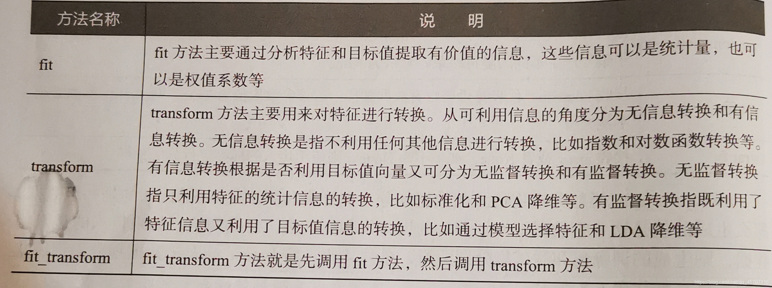
sklearn將相關的功能封裝爲轉換器,轉換器主要包含有3個方法:fit、transform、fit_trainsform:
import numpy as np
from sklearn.preprocessing import MinMaxScaler

# 生成規則
Scaler = MinMaxScaler().fit(cancer_data_train)
# 將規則應用於訓練集
cancer_trainScaler = Scaler.transform(cancer_data_train)
# 將規則應用於測試集
cancer_testScaler = Scaler.transform(cancer_data_test)

print('離差標準化前訓練集數據的最小值:',cancer_data_train.min())
print('離差標準化後訓練集數據的最小值:',np.min(cancer_trainScaler))
print('離差標準化前訓練集數據的最大值:',np.max(cancer_data_train))
print('離差標準化後訓練集數據的最大值:',np.max(cancer_trainScaler))
print('離差標準化前測試集數據的最小值:',np.min(cancer_data_test))
print('離差標準化後測試集數據的最小值:',np.min(cancer_testScaler))
print('離差標準化前測試集數據的最大值:',np.max(cancer_data_test))
print('離差標準化後測試集數據的最大值:',np.max(cancer_testScaler))
離差標準化前訓練集數據的最小值: 0.0
離差標準化後訓練集數據的最小值: 0.0
離差標準化前訓練集數據的最大值: 4254.0
離差標準化後訓練集數據的最大值: 1.0000000000000002
離差標準化前測試集數據的最小值: 0.0
離差標準化後測試集數據的最小值: -0.057127602776294695
離差標準化前測試集數據的最大值: 3432.0
離差標準化後測試集數據的最大值: 1.3264399566986453
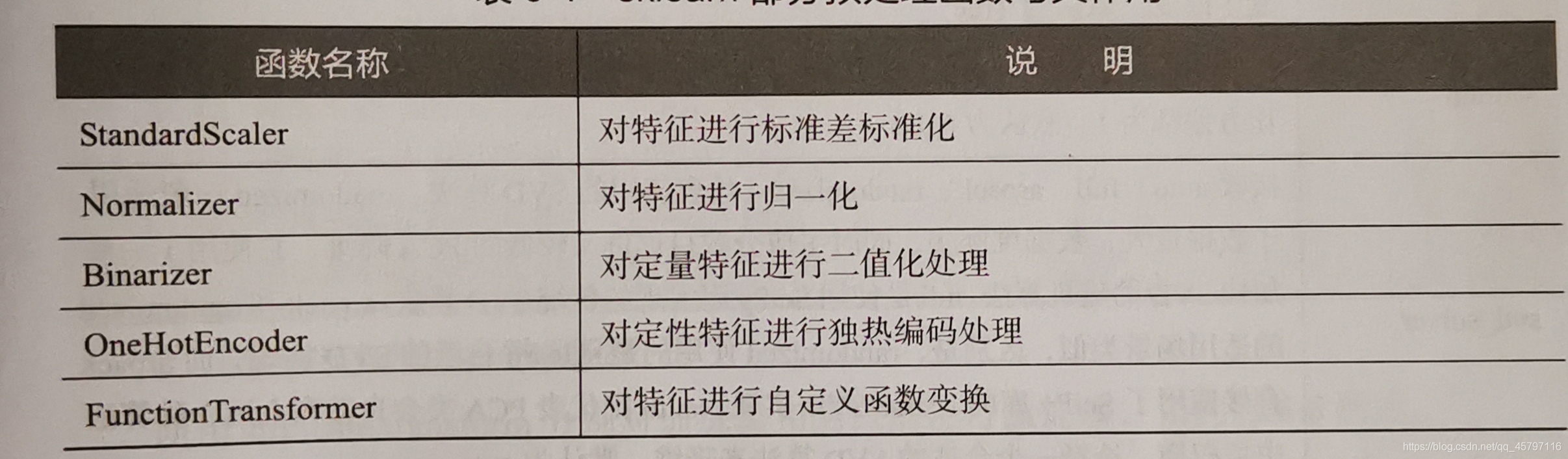
目前利用sklearn能夠實現對傳入的numpy陣列進行標準化處理、歸一化處理、、二值化處理和PCA降維處理。前面基於pandas庫介紹的標準化處理在日常數據分析過程中,各類特徵處理相關的操作都需要對訓練集和測試集分開進行,需要將訓練集中的操作規則、權重係數等應用到測試集中,利用pandas會使得過程繁瑣,而sklearn轉換器可以輕鬆實現。
除了上面展示的離差標準化函數MinMaxScaler外,還提供了一系列的數據預處理常式:
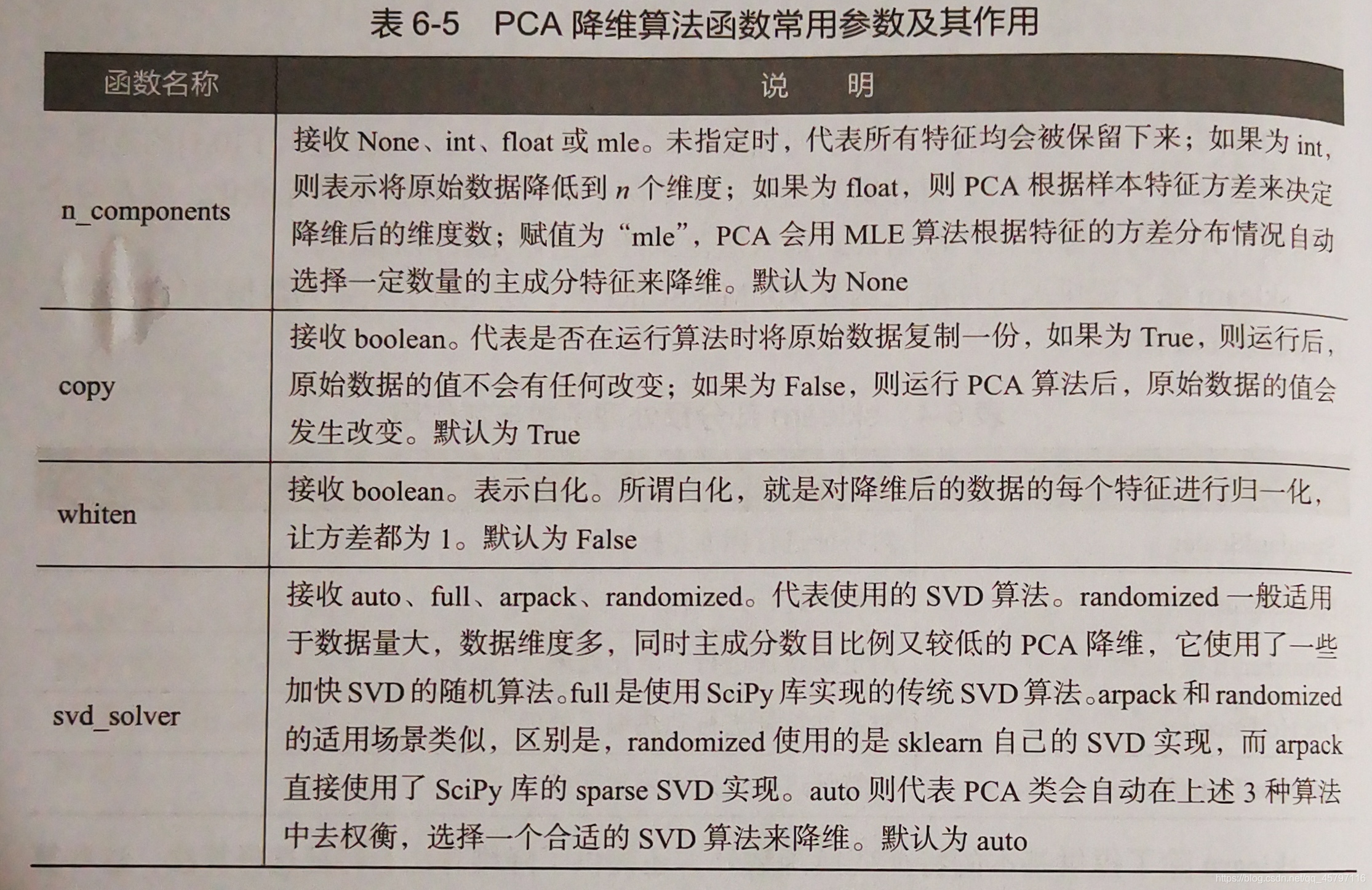
PCA降維處理:
sklearn.decomposition.PCA(n_components=None, *, copy=True, whiten=False, svd_solver='auto', tol=0.0, iterated_power='auto', random_state=None)
from sklearn.decomposition import PCA

# 生成規則
pca_model=PCA(n_components=10).fit(cancer_trainScaler)
# 將規則應用到訓練集
cancer_trainPca = pca_model.transform(cancer_trainScaler)
# 將規則應用到測試集
cancer_testPca = pca_model.transform(cancer_testScaler)

print('PCA降維前訓練集數據的形狀爲:',cancer_trainScaler.shape)
print('PCA降維後訓練集數據的形狀爲:',cancer_trainPca.shape)
print('PCA降維前測試集數據的形狀爲:',cancer_testScaler.shape)
print('PCA降維後測試集數據的形狀爲:',cancer_testPca.shape)
PCA降維前訓練集數據的形狀爲: (455, 30)
PCA降維後訓練集數據的形狀爲: (455, 10)
PCA降維前測試集數據的形狀爲: (114, 30)
PCA降維後測試集數據的形狀爲: (114, 10)
二、構建評價聚類模型
聚類分析是在沒有給定劃分類別的情況下,根據數據相似度進行樣本分組的一種方法。
1.使用sklearn估計器構建聚類模型
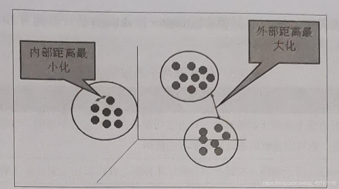
聚類的輸入是一組未被標記的樣本,聚類根據數據自身的距離或相似度將它們劃分爲若幹組,劃分的原則是:組內距離最小化,組間距離最大化。
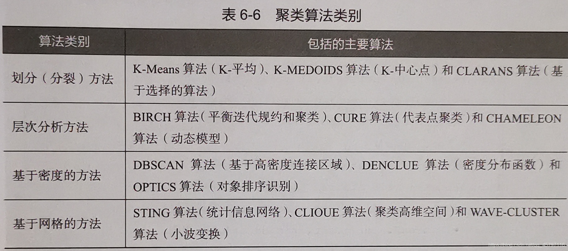
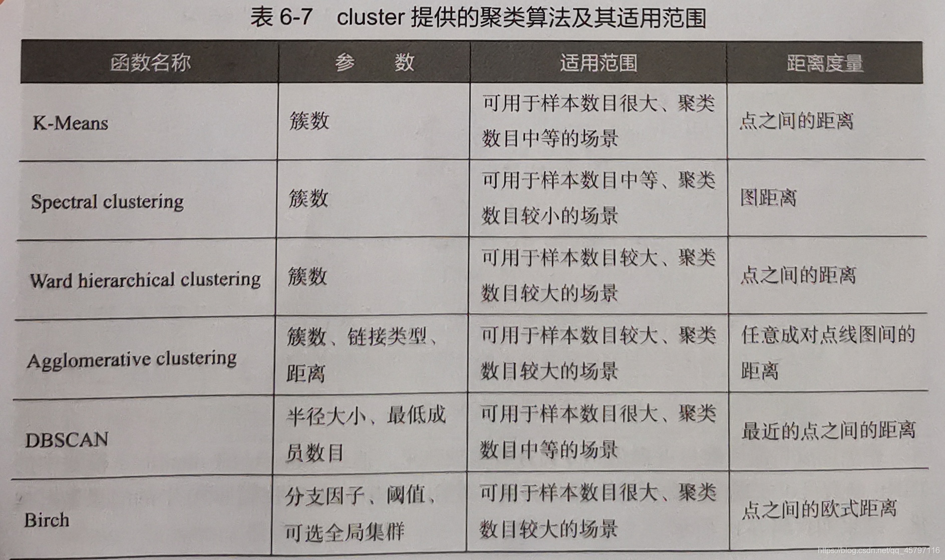
sklearn常用的聚類演算法模組cluster提供的聚類演算法:
聚類演算法的實現需要sklearn估計器(Estimnator),其擁有fit和predict兩個方法:
| 方法名稱 | 說明 |
|---|---|
| fit | fit方法主要適用於訓練演算法。該方法可以有效接收用於有監督學習的訓練集及其標籤兩個參數,也可以接收用於無監督學習的數據 |
| predict | 用於預測有監督學習的測試集標籤,也可以用於劃分傳入數據的類別 |
以iris數據爲例,使用sklearn估計器構建K-Means聚類模型:
from sklearn.datasets import load_iris
from sklearn.preprocessing import MinMaxScaler
from sklearn.cluster import KMeans

iris = load_iris()           # 載入iris數據集
iris_data = iris['data']     # 提取iris數據集中的特徵
iris_target = iris['target'] # 提取iris數據集中的標籤
iris_feature_names = iris['feature_names'] #提取iris數據集中的特徵名稱

scale = MinMaxScaler().fit(iris_data) # 對數據集中的特徵設定訓練規則
iris_dataScale = scale.transform(iris_data) # 應用規則

kmeans = KMeans(n_clusters=3,random_state=123).fit(iris_dataScale) # 構建並訓練模型
print('構建的K-Means模型爲:\n',kmeans)
#構建的K-Means模型爲:
 KMeans(algorithm='auto', copy_x=True, init='k-means++', max_iter=300,
       n_clusters=3, n_init=10, n_jobs=None, precompute_distances='auto',
       random_state=123, tol=0.0001, verbose=0)
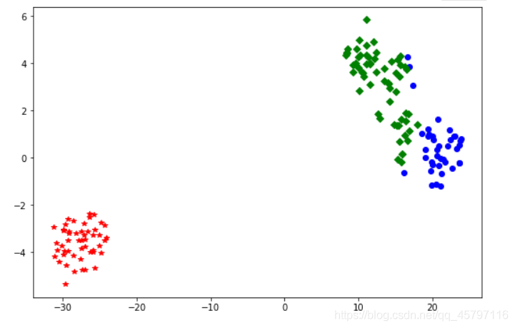
聚類完成後可以通過sklearn的manifold模組中的TXNE函數實現多維數據的視覺化展現。
import pandas as pd
from sklearn.manifold import TSNE
import matplotlib.pyplot as plt

# 使用TSNE進行數據降維,降成2維
tsne = TSNE(n_components=2,init='random',random_state=177).fit(iris_data)

df = pd.DataFrame(tsne.embedding_) # 將原始數據轉換爲DataFrame
df['labels'] = kmeans.labels_ # 將聚類結果儲存進df數據表

# 提取不同標籤的數據
df1 = df[df['labels']==0]
df2 = df[df['labels']==1]
df3 = df[df['labels']==2]

# 繪製圖形
# 繪製畫布大小
fig = plt.figure(figsize=(9,6))
# 用不同顏色表示不同數據
plt.plot(df1[0],df1[1],'bo',df2[0],df2[1],'r*',df3[0],df3[1],'gD')
# 儲存圖片
plt.savefig('tmp/聚類結果.png')
# 展示
plt.show()
2.評價聚類模型
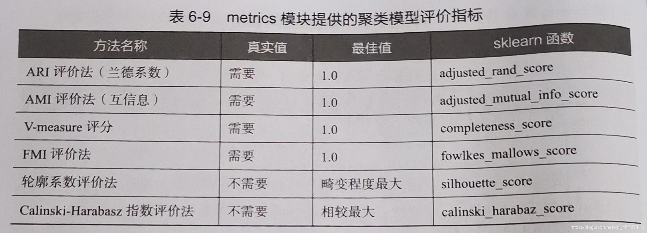
聚類評價的標準是組內的物件相互之間是相似的,而不同組間的物件是不同的,即組內相似性越大,組間差別性越大,聚類效果越好。
注意:
1.前四種方法需要真實值的配合才能 纔能夠評價聚類演算法的優劣,更具有說服力,並且在實際操作中,有真實值參考下,聚類方法的評價可以等同於分類演算法的評價。
2.除了輪廓係數評價法以外的評價方法,在不考慮業務場景的情況下都是分數越高越好,最高分爲1,而輪廓係數評價法需要判斷不同類別數目情況下的輪廓係數的走勢,尋找最優的聚類數目。
FMI評價法
from sklearn.datasets import load_iris

iris = load_iris()           # 載入iris數據集
iris_data = iris['data']     # 提取數據集特徵
iris_target = iris['target'] # 提取數據集標籤

from sklearn.metrics import fowlkes_mallows_score from sklearn.cluster
import KMeans

for i in range(2,7):
    # 構建並訓練模型
    kmeans = KMeans(n_clusters=i,random_state=123).fit(iris_data)
    score = fowlkes_mallows_score(iris_target,kmeans.labels_)
    print('iris數據聚%d類FMI評價分值爲:%f'%(i,score))

iris數據聚2類FMI評價分值爲:0.750473 iris數據聚3類FMI評價分值爲:0.820808
iris數據聚4類FMI評價分值爲:0.756593 iris數據聚5類FMI評價分值爲:0.725483
iris數據聚6類FMI評價分值爲:0.614345 ```
通過結果可以看出來,當聚類爲3時FMI評價分最高,所以當聚類3的時候,K-Means模型最好。
輪廓係數評價法
from sklearn.datasets import load_iris

iris = load_iris()           # 載入iris數據集
iris_data = iris['data']     # 提取數據集特徵
iris_target = iris['target'] # 提取數據集標籤

from sklearn.metrics import silhouette_score from sklearn.cluster
import KMeans import matplotlib.pyplot as plt

silhouettteScore = [] for i in range(2,15):
    ##構建並訓練模型
    kmeans = KMeans(n_clusters = i,random_state=123).fit(iris_data)
    score = silhouette_score(iris_data,kmeans.labels_)
    silhouettteScore.append(score) plt.figure(figsize=(10,6)) plt.plot(range(2,15),silhouettteScore,linewidth=1.5, linestyle="-")
plt.show() ```
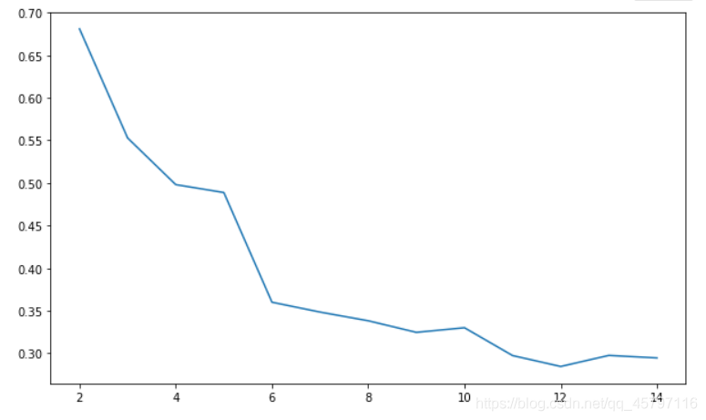
從圖形可以看出,聚類數目爲2、3和5、6時平均畸變程度最大。由於iris數據本身就是3種鳶尾花的花瓣、花萼長度和寬度的數據,側面說明了聚類數目爲3的時候效果最佳。
Calinski_Harabasz指數評價法
from sklearn.datasets import load_iris

iris = load_iris()           # 載入iris數據集
iris_data = iris['data']     # 提取數據集特徵
iris_target = iris['target'] # 提取數據集標籤

from sklearn.metrics import silhouette_score
from sklearn.cluster import KMeans
from sklearn.metrics import calinski_harabasz_score

for i in range(2,7):
    ##構建並訓練模型
    kmeans = KMeans(n_clusters = i,random_state=123).fit(iris_data)
    score = calinski_harabasz_score(iris_data,kmeans.labels_)
    print('iris數據聚%d類calinski_harabaz指數爲:%f'%(i,score))

iris數據聚2類calinski_harabaz指數爲:513.924546
iris數據聚3類calinski_harabaz指數爲:561.627757
iris數據聚4類calinski_harabaz指數爲:530.765808
iris數據聚5類calinski_harabaz指數爲:495.541488
iris數據聚6類calinski_harabaz指數爲:469.836633 ```
同樣可以看出在聚類爲3時,K-Means模型爲最優。
綜合以上評價方法的使用,在有真實值參考時,幾種方法都能有效的展示評估聚合模型;在沒有真實值參考時,可以將輪廓係數評價與Calinski_Harabasz指數評價相結合使用。
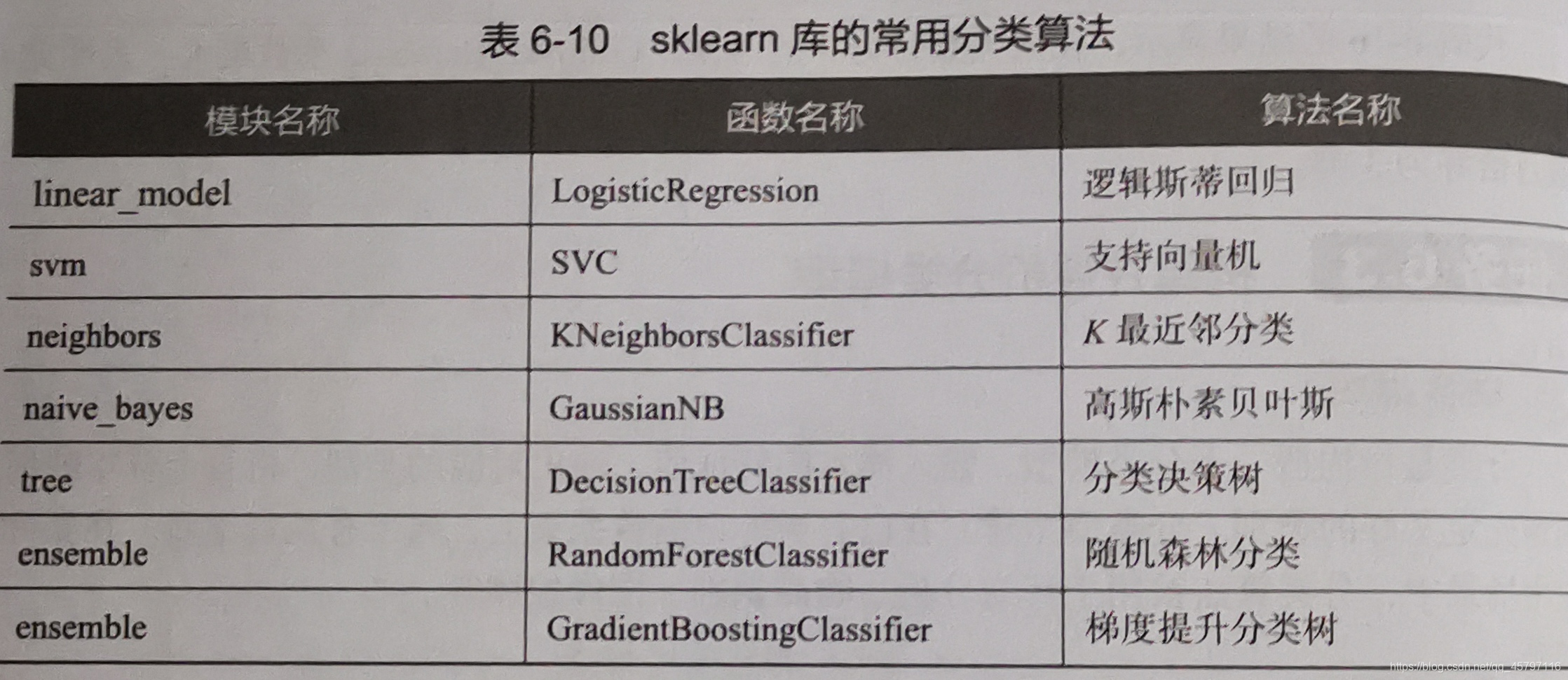
三、構建評價分類模型
分類是指構造一個分類模型,輸入樣本的特徵值,輸出對應類別,將每個樣本對映到預先定義好的類別。分類模型是建立在自己已有類標記的數據集上,屬於有監督學習。在實際應用場景中,分類演算法被應用在行爲分析、物品識別、影象檢測等。
1.使用sklearn估計器構建分類模型
以breast_cancer數據集爲例,使用sklearn估計器構建支援向量機(SVM)模型:
import numpy as np
from sklearn.datasets import load_breast_cancer
from sklearn.svm import SVC
from sklearn.model_selection import train_test_split
from sklearn.preprocessing import StandardScaler

cancer = load_breast_cancer()
cancer_data = cancer['data']
cancer_target = cancer['target']
cancer_names = cancer['feature_names']

## 將數據劃分爲訓練集測試集
cancer_data_train,cancer_data_test,cancer_target_train,cancer_target_test = \
train_test_split(cancer_data,cancer_target,test_size = 0.2,random_state = 22)

## 數據標準化
stdScaler = StandardScaler().fit(cancer_data_train)      # 設定標準化規則
cancer_trainStd = stdScaler.transform(cancer_data_train) # 將標準化規則應用到訓練集
cancer_testStd = stdScaler.transform(cancer_data_test)   # 將標準化規則應用到測試集

## 建立SVM模型
svm = SVC().fit(cancer_trainStd,cancer_target_train)
print('建立的SVM模型爲:\n',svm)
#建立的SVM模型爲:
 SVC(C=1.0, break_ties=False, cache_size=200, class_weight=None, coef0=0.0,
    decision_function_shape='ovr', degree=3, gamma='scale', kernel='rbf',
    max_iter=-1, probability=False, random_state=None, shrinking=True,
    tol=0.001, verbose=False)

## 預測訓練集結果
cancer_target_pred = svm.predict(cancer_testStd)
print('預測前20個結果爲:\n',cancer_target_pred[:20])
#預測前20個結果爲:
 [1 0 0 0 1 1 1 1 1 1 1 1 0 1 1 1 0 0 1 1]
## 求出預測和真實一樣的數目
true = np.sum(cancer_target_pred == cancer_target_test )
print('預測對的結果數目爲:', true)
print('預測錯的的結果數目爲:', cancer_target_test.shape[0]-true)
print('預測結果準確率爲:', true/cancer_target_test.shape[0])
預測對的結果數目爲: 111
預測錯的的結果數目爲: 3
預測結果準確率爲: 0.9736842105263158
2.評價分類模型
分類模型對測試集進行預測而得出的準確率並不能很好地反映模型的效能,爲了有效判斷一個預測模型的效能表現,需要結合真實值計算出精確率、召回率、F1值、Cohen’s Kappa係數等指標來衡量。
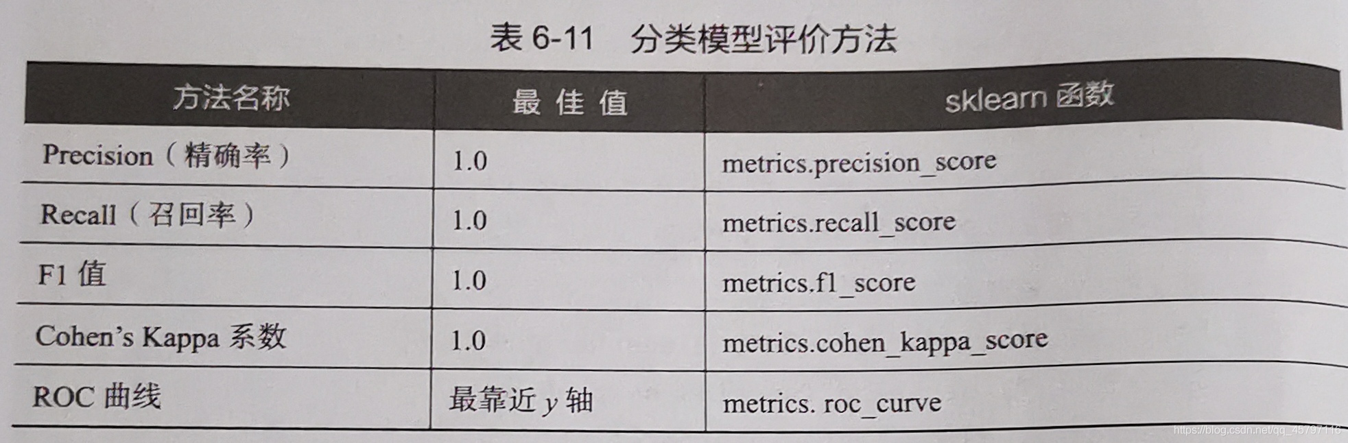
使用單一評價指標(Precision、Recall、F1值、Cohen’s Kappa係數)
from sklearn.metrics import accuracy_score,precision_score,recall_score,f1_score,cohen_kappa_score

print('使用SVM預測breast_cancer數據的準確率爲:',
      accuracy_score(cancer_target_test,cancer_target_pred))
print('使用SVM預測breast_cancer數據的精確率爲:',
      precision_score(cancer_target_test,cancer_target_pred))
print('使用SVM預測breast_cancer數據的召回率爲:',
      recall_score(cancer_target_test,cancer_target_pred))
print('使用SVM預測breast_cancer數據的F1值爲:',
      f1_score(cancer_target_test,cancer_target_pred))
print('使用SVM預測breast_cancer數據的Cohen’s Kappa係數爲:',
      cohen_kappa_score(cancer_target_test,cancer_target_pred))
使用SVM預測breast_cancer數據的準確率爲: 0.9736842105263158
使用SVM預測breast_cancer數據的精確率爲: 0.9594594594594594
使用SVM預測breast_cancer數據的召回率爲: 1.0
使用SVM預測breast_cancer數據的F1值爲:0.9793103448275862
使用SVM預測breast_cancer數據的Cohen’s Kappa係數爲: 0.9432082364662903 ```
sklearn模組除了提供了Precision等單一評價指標外,還提供了一個能夠輸出分類模型評價報告的函數classification_report:
classification_report參數詳解~python sklearn.metrics.classification_report(y_true, y_pred, *, labels=None, target_names=None, sample_weight=None, digits=2, output_dict=False, zero_division='warn')print('使用SVM預測iris數據的分類報告爲:\n', classification_report(cancer_target_test,cancer_target_pred)) #使用SVM預測iris數據的分類報告爲: precision recall f1-score support 0 1.00 0.93 0.96 43 1 0.96 1.00 0.98 71 accuracy 0.97 114 macro avg 0.98 0.97 0.97 114 weighted avg 0.97 0.97 0.97 114 ```
繪製ROC曲線
from sklearn.metrics import roc_curve
import matplotlib.pyplot as plt

## 求出ROC曲線的x軸和y軸
fpr, tpr, thresholds = roc_curve(cancer_target_test,cancer_target_pred)
# 設定畫布
plt.figure(figsize=(10,6))

plt.xlim(0,1) ##設定x軸的範圍
plt.ylim(0.0,1.1) ## 設定y軸的範圍
plt.xlabel('FalsePostive Rate')
plt.ylabel('True Postive Rate')

x = [0,0.2,0.4,0.6,0.8,1]
y = [0,0.2,0.4,0.6,0.8,1]

# 繪圖
plt.plot(x,y,linestyle='-.',color='green')
plt.plot(fpr,tpr,linewidth=2, linestyle="-",color='red')
# 展示
plt.show()
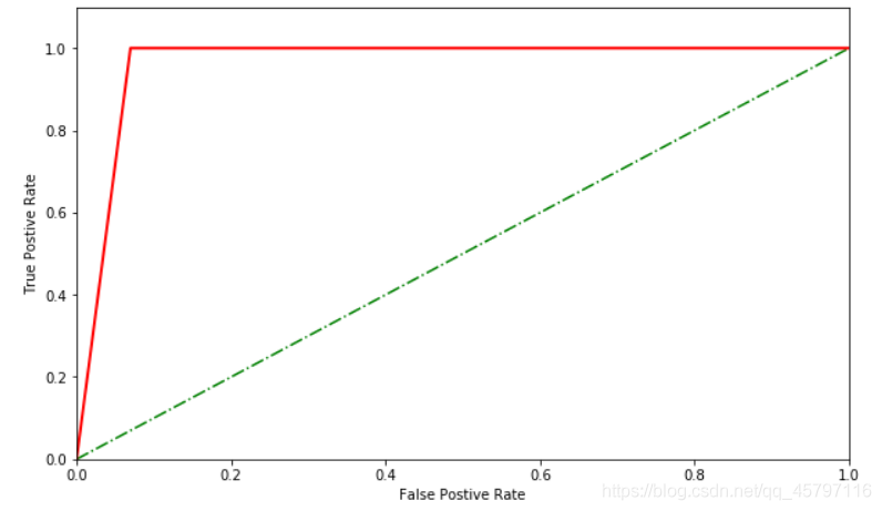
ROC曲線橫縱座標範圍是[0,1],通常情況下,ROC曲線與x軸形成的面積越大,表示模型效能越好。當ROC曲線如虛線所示時,表明模型的計算結果基本都是隨機得來的,此時模型起到的作用幾乎爲0.
四、構建評價迴歸模型
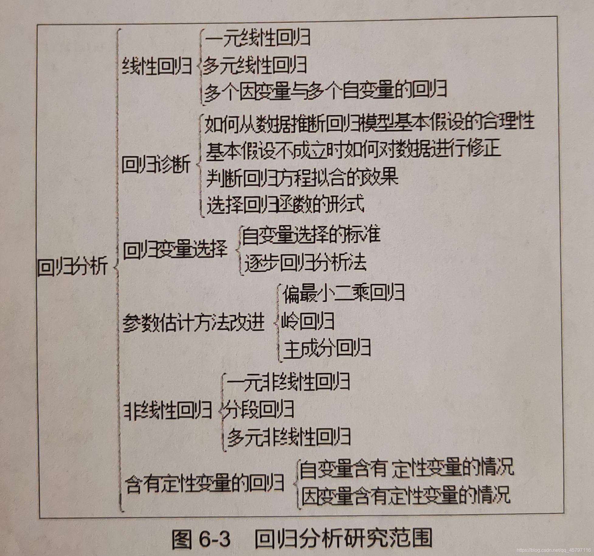
迴歸演算法的實現過程與分類演算法相似,原理相差不大。分類和迴歸的主要區別在於,分類演算法的標籤是離散的,但是迴歸演算法的標籤是連續的。迴歸演算法在交通、物流、社交、網路等領域發揮作用巨大。
1.使用sklearn估計器構建迴歸模型
在迴歸模型中,自變數和因變數具有相關關係,自變數的值是已知的,因變數的值是要預測的。迴歸演算法的實現步驟和分類演算法基本相同,分爲學習和預測兩個步驟。
學習:通過訓練樣本來擬合迴歸方程
預測:利用學習過程中擬合出的方程,將測試數據放入方程中求出預測值。

from sklearn.datasets import load_boston
from sklearn.model_selection import train_test_split
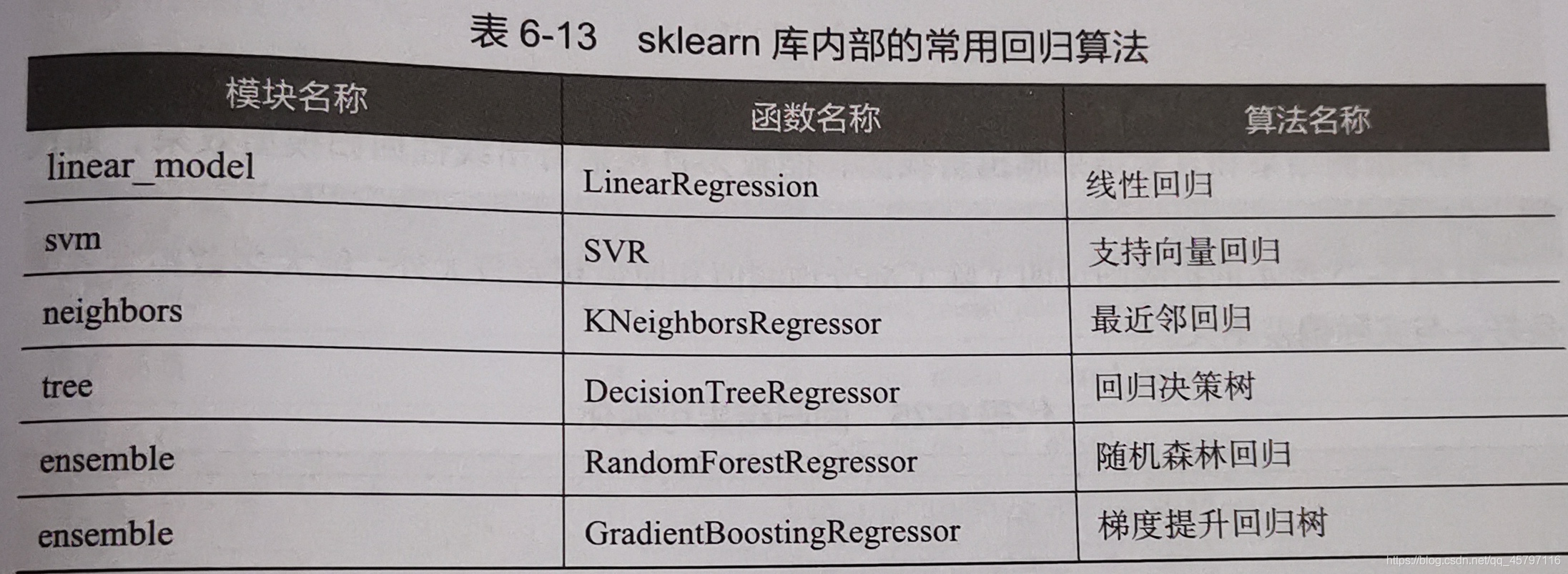
from sklearn.linear_model import LinearRegression
# 載入boston數據集
boston = load_boston()
# 提取數據
x = boston['data']
y = boston['target']
names = boston['feature_names']
# 將數據劃分爲訓練集和測試集
x_train,x_test,y_train,y_test=train_test_split(x,y,test_size=0.2,random_state=125)
# 建立線性迴歸模型
clf = LinearRegression().fit(x_train,y_train)
print('建立的Linear Regression模型爲:\n',clf)
#建立的 Linear Regression模型爲:
LinearRegression(copy_X=True, fit_intercept=True, n_jobs=None, normalize=False)
# 預測測試集結果
y_pred = clf.predict(x_test)
print('預測前20個結果爲:\n',y_pred[:20])
#預測前20個結果爲:
[21.16289134 19.67630366 22.02458756 24.61877465 14.44016461 23.32107187
16.64386997 14.97085403 33.58043891 17.49079058 25.50429987 36.60653092
25.95062329 28.49744469 19.35133847 20.17145783 25.97572083 18.26842082
16.52840639 17.08939063]
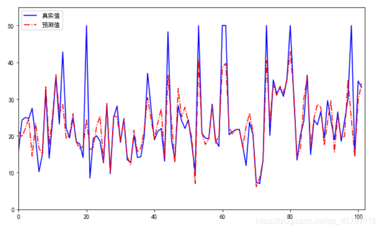
迴歸結果視覺化
# 迴歸結果視覺化
import matplotlib.pyplot as plt
from matplotlib import rcParams

# 設定中文顯示
rcParams['font.sans-serif'] = 'SimHei'

# 設定畫布
plt.figure(figsize=(10,6))

# 繪圖
plt.plot(range(y_test.shape[0]),y_test,color='blue',linewidth=1.5,linestyle='-')
plt.plot(range(y_test.shape[0]),y_pred,color='red',linewidth=1.5,linestyle='-.')

# 設定影象屬性
plt.xlim((0,102))
plt.ylim((0,55))
plt.legend(['真實值','預測值'])

# 儲存圖片
plt.savefig('tmp/聚迴歸類結果.png')

#展示
plt.show()
2.評價迴歸模型
迴歸模型的效能評價不同於分類模型,雖然都是對照真實值進行評價,但是由於迴歸模型的預測結果和真實值都是連續地,所以不能夠用之前的精確率、召回率、F1值進行評價。
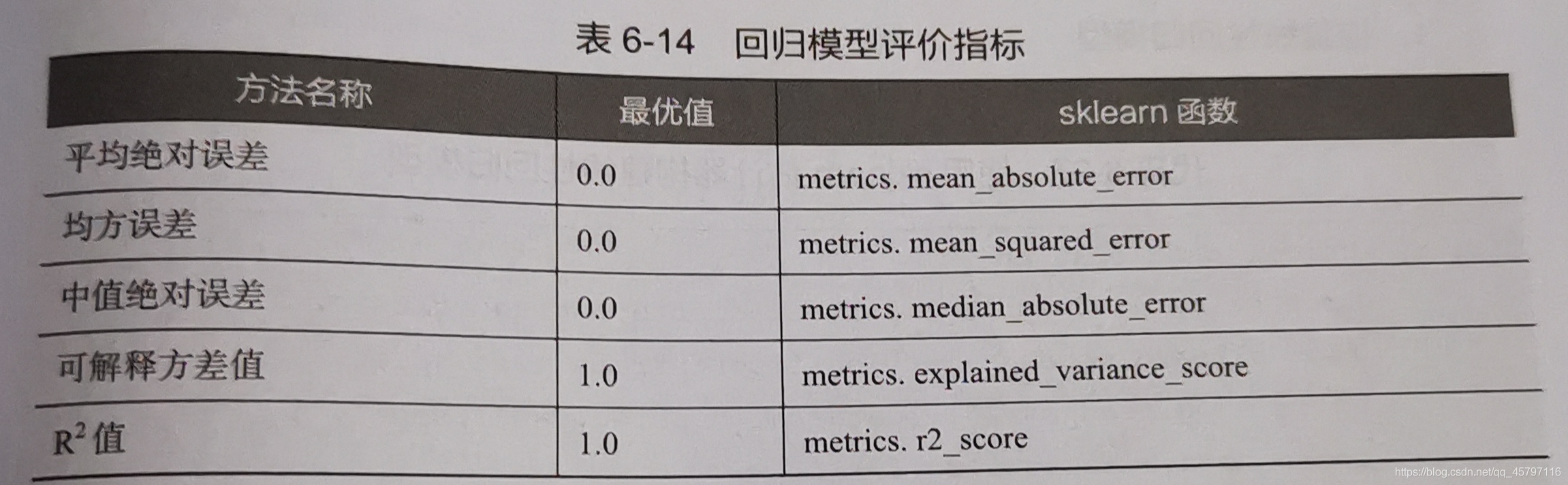
使用explained_variance_score, mean_absolute_error, mean_squared_error, r2_score, median_absolute_error進行迴歸評價
from sklearn.metrics import explained_variance_score,mean_absolute_error,mean_squared_error,\
median_absolute_error,r2_score
print('Boston數據線性迴歸模型的平均絕對誤差爲:',
     mean_absolute_error(y_test,y_pred))
print('Boston數據線性迴歸模型的均方誤差爲:',
     mean_squared_error(y_test,y_pred))
print('Boston數據線性迴歸模型的中值絕對誤差爲:',
     median_absolute_error(y_test,y_pred))
print('Boston數據線性迴歸模型的可解釋方差值爲:',
     explained_variance_score(y_test,y_pred))
print('Boston數據線性迴歸模型的R方值爲:',
     r2_score(y_test,y_pred))
#Boston數據線性迴歸模型的平均絕對誤差爲: 3.3775517360082032
#Boston數據線性迴歸模型的均方誤差爲: 31.15051739031563
#Boston數據線性迴歸模型的中值絕對誤差爲: 1.7788996425420773
#Boston數據線性迴歸模型的可解釋方差值爲: 0.710547565009666
#Boston數據線性迴歸模型的R方值爲: 0.7068961686076838