深度學習之識別貓（深度之眼assignment 1）
搭建好了深度學習的學習環境，在Ubuntu上開啓iPython notebook進行學習。
首先關於邏輯迴歸，sigmoid函數。

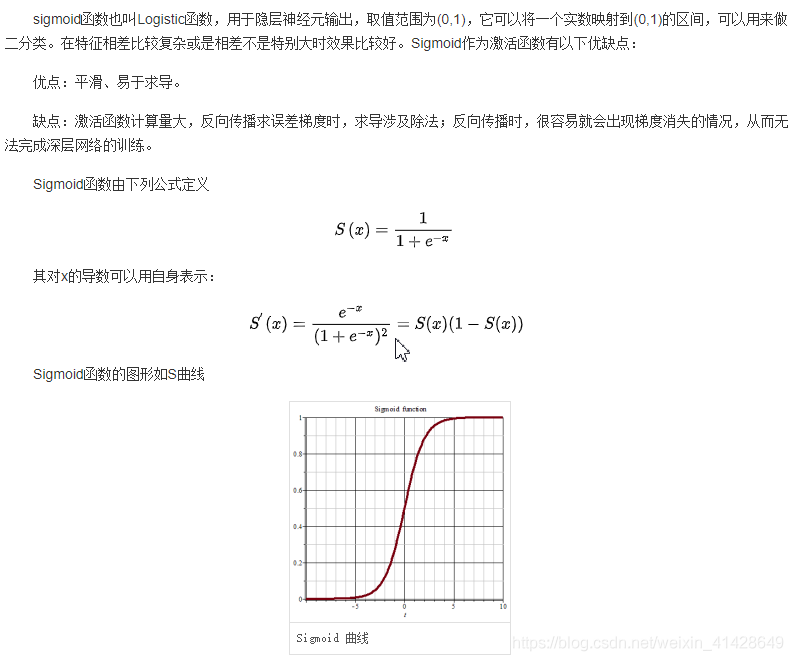
程式碼實現如下：

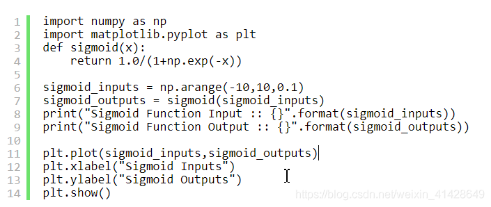
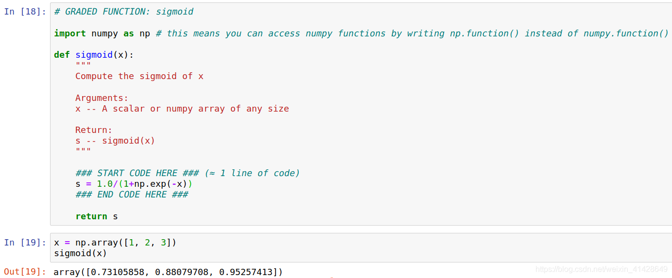
然後自己在jupyter notebook裏面敲了程式碼進行實現。

計算斜率，即求導：

numpy庫shape和reshape的用法

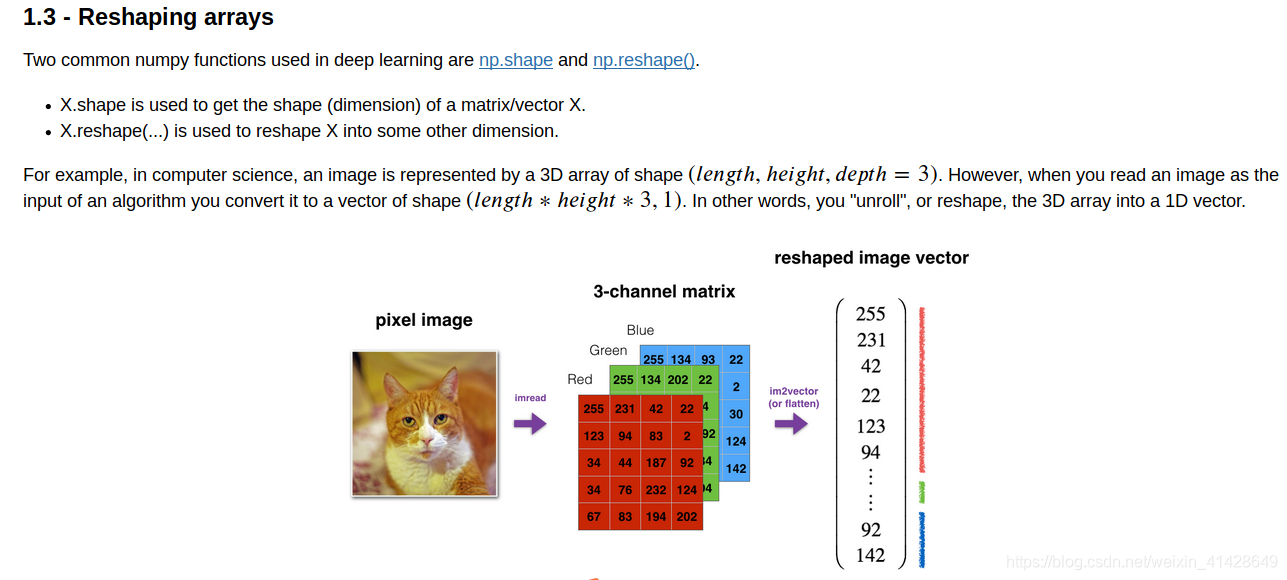
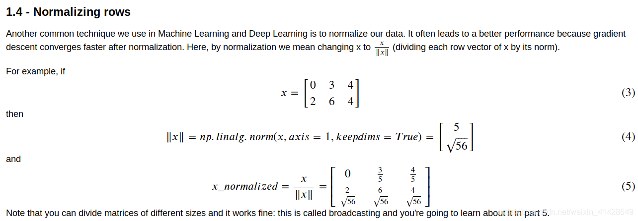
線上代裏面學的標準化等也是會用到

下面 下麪運用邏輯迴歸來實現一個專案：識別圖片是否爲貓。
import numpy as np
import matplotlib.pyplot as plt
import h5py
import scipy
from PIL import Image
from scipy import ndimage
from lr_utils import load_dataset

%matplotlib inline #對於這一行，如果不是用notebook的話可以去掉

Loading the data (cat/non-cat)

train_set_x_orig, train_set_y, test_set_x_orig, test_set_y, classes = load_dataset()
如下是對這行程式碼的解析
「」"
print(train_set_x_orig.shape)
print(train_set_y.shape)
print(test_set_x_orig.shape)
print(test_set_y.shape)
print(classes)
「」"
輸出爲：
(209, 64, 64, 3)
(1, 209)
(50, 64, 64, 3)
(1, 50)
[b’non-cat’ b’cat’]

Example of a picture

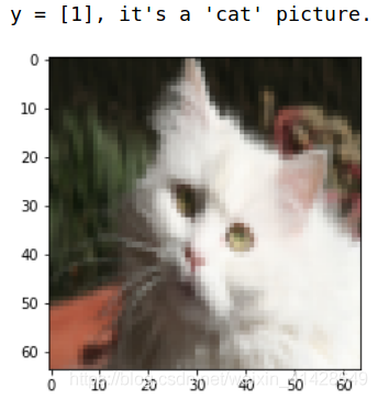
index = 102
plt.imshow(train_set_x_orig[index])
print ("y = " + str(train_set_y[:, index]) + 「, it’s a '」 + classes[np.squeeze(train_set_y[:, index])].decode(「utf-8」) + 「’ picture.」)

下面 下麪是呼叫參數的練習：

m_train = train_set_x_orig.shape[0]
m_test = test_set_x_orig.shape[0]
num_px = train_set_x_orig.shape[2]

print ("Number of training examples: m_train = " + str(m_train))
print ("Number of testing examples: m_test = " + str(m_test))
print ("Height/Width of each image: num_px = " + str(num_px))
print (「Each image is of size: (」 + str(num_px) + ", " + str(num_px) + 「, 3)」)
print ("train_set_x shape: " + str(train_set_x_orig.shape))
print ("train_set_y shape: " + str(train_set_y.shape))
print ("test_set_x shape: " + str(test_set_x_orig.shape))
print ("test_set_y shape: " + str(test_set_y.shape))
輸出爲：
Number of training examples: m_train = 209
Number of testing examples: m_test = 50
Height/Width of each image: num_px = 64
Each image is of size: (64, 64, 3)
train_set_x shape: (209, 64, 64, 3)
train_set_y shape: (1, 209)
test_set_x shape: (50, 64, 64, 3)
test_set_y shape: (1, 50)

Exercise: Reshape the training and test data sets so that images of size (num_px, num_px, 3) are flattened into single vectors of shape (num_px ∗ num_px ∗3, 1).
A trick when you want to flatten a matrix X of shape (a,b,c,d) to a matrix X_flatten of shape (b∗c∗d, a) is to use:
X_flatten = X.reshape(X.shape[0], -1).T # X.T is the transpose of X
#即把每張圖片展開成向量。

Reshape the training and test examples

train_set_x_flatten = train_set_x_orig.reshape(train_set_x_orig.shape[0], -1).T
test_set_x_flatten = test_set_x_orig.reshape(test_set_x_orig.shape[0], -1).T
‘’’
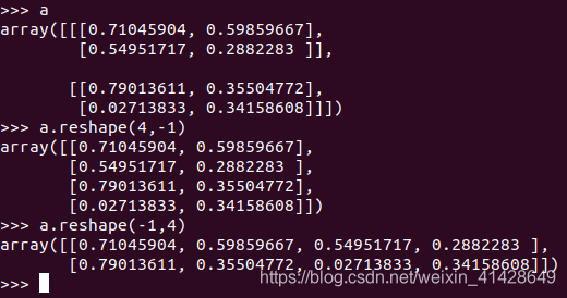
這裏要注意reshape的順序
train_set_x_flatten = train_set_x_orig.reshape( -1,train_set_x_orig.shape[0]).T
其中-1是能夠自動計算行列
執行程式碼後，在畫素檢查那裏是略有區別的

‘’’

print ("train_set_x_flatten shape: " + str(train_set_x_flatten.shape))
print ("train_set_y shape: " + str(train_set_y.shape))
print ("test_set_x_flatten shape: " + str(test_set_x_flatten.shape))
print ("test_set_y shape: " + str(test_set_y.shape))
print ("sanity check after reshaping: " + str(train_set_x_flatten[0:5,0]))

Output:
train_set_x_flatten shape: (12288, 209)
train_set_y shape: (1, 209)
test_set_x_flatten shape: (12288, 50)
test_set_y shape: (1, 50)
sanity check after reshaping: [17 31 56 22 33]

To represent color images, the red, green and blue channels (RGB) must be specified for each pixel, and so the pixel value is actually a vector of three numbers ranging from 0 to 255.
One common preprocessing step in machine learning is to center and standardize your dataset, meaning that you substract the mean of the whole numpy array from each example, and then divide each example by the standard deviation of the whole numpy array. But for picture datasets, it is simpler and more convenient and works almost as well to just divide every row of the dataset by 255 (the maximum value of a pixel channel).

train_set_x = train_set_x_flatten/255.
test_set_x = test_set_x_flatten/255.
把畫素的值壓縮到0～1

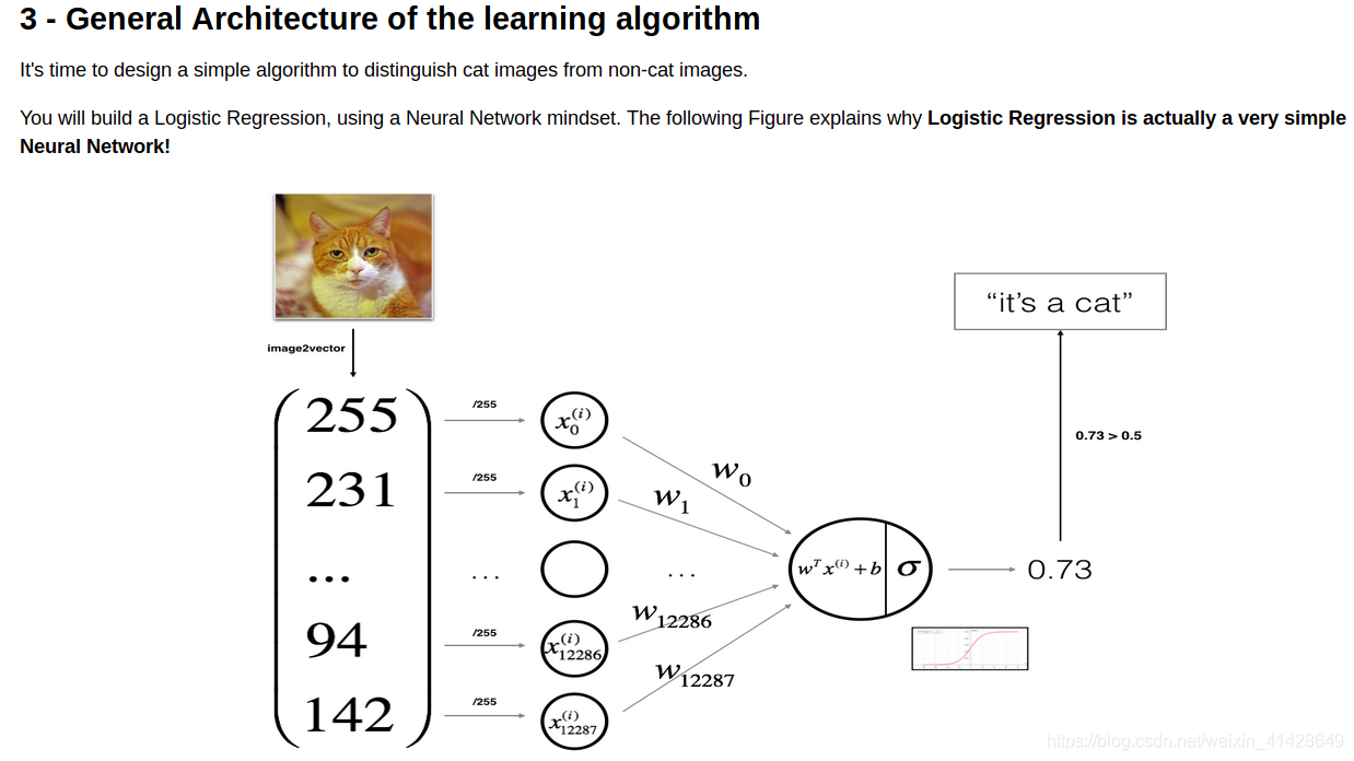
如下是整個流程的圖示以及相關公式：

GRADED FUNCTION: sigmoid

def sigmoid(z):
「」"
Compute the sigmoid of z

Arguments:
z – A scalar or numpy array of any size.#這裏是難點，既要標量，又要numpy陣列

Return:
s – sigmoid(z)
「」"

s = 1.0/(1+np.exp(-z))   #使用numpy的內建函數
return s

print ("sigmoid([0, 2]) = " + str(sigmoid(np.array([0,2]))))
Output:
sigmoid([0, 2]) = [0.5 0.88079708]

函數初始化部分：

GRADED FUNCTION: initialize_with_zeros

def initialize_with_zeros(dim):
「」"
This function creates a vector of zeros of shape (dim, 1) for w and initializes b to 0.

Argument:
dim -- size of the w vector we want (or number of parameters in this case)

Returns:
w -- initialized vector of shape (dim, 1)
b -- initialized scalar (corresponds to the bias)
"""

### START CODE HERE ### (≈ 1 line of code)
w = np.zeros((dim,1))
b = 0
### END CODE HERE ###

assert(w.shape == (dim, 1))
assert(isinstance(b, float) or isinstance(b, int))

return w, b

dim = 2
w, b = initialize_with_zeros(dim)
print ("w = " + str(w))
print ("b = " + str(b))

Output:
w = [[0.]
[0.]]
b = 0

前向傳播和反向傳播：

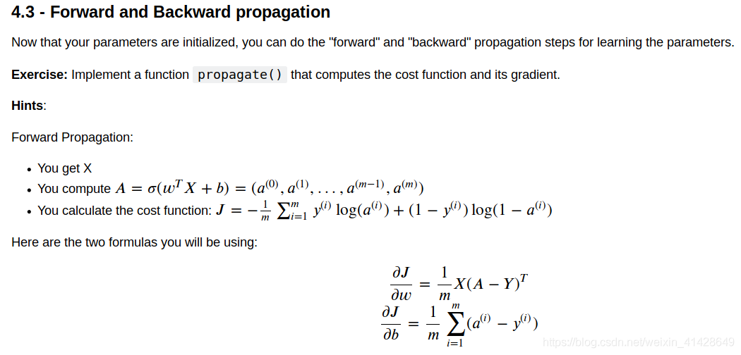
前向傳播：

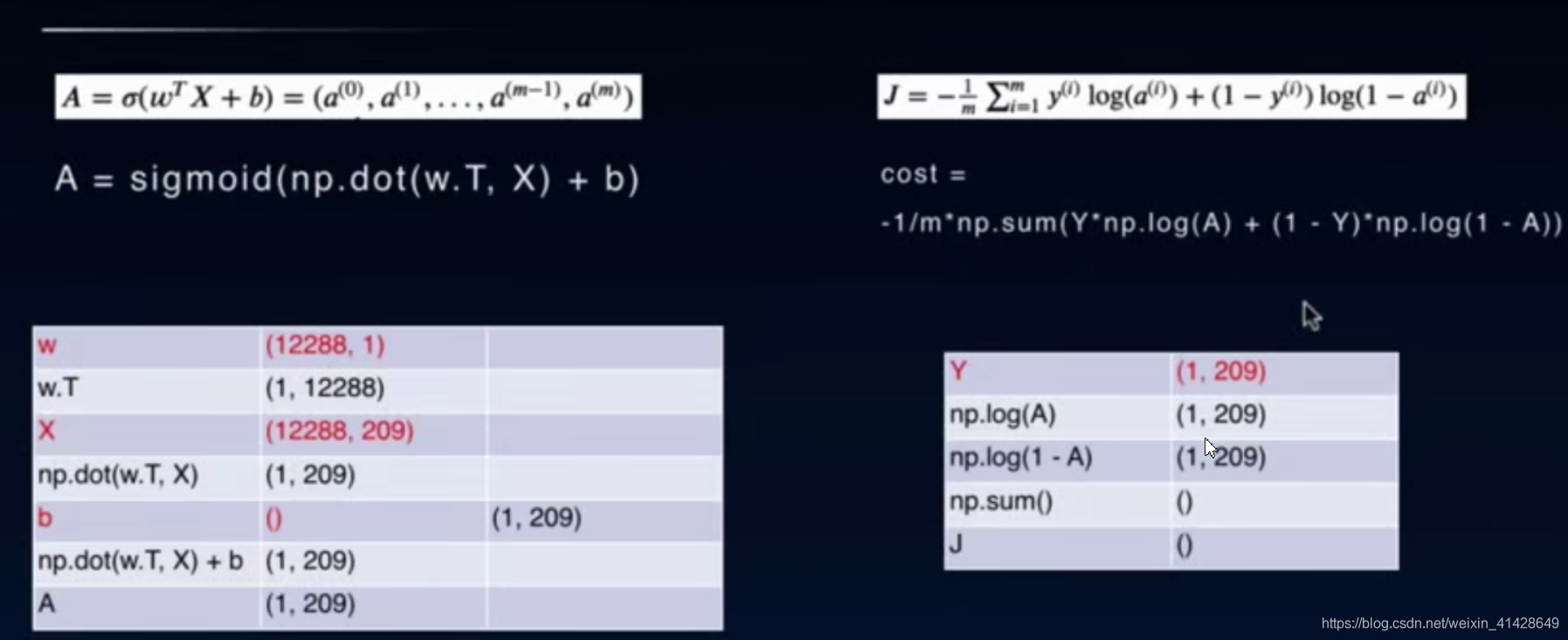
左邊：
w = （12288,1） #12288 = 64 * 64 * 3
w.T是轉置，np.dot(w.T,X)是將X和w.T點乘，然後得到的數直接加b(標量)
經過sigmoid函數之後把w參數更新到最優，A就是我們對X的預測結果
在後面編寫predict方程的時候，也會用到這個公式
右邊：
分層運算，數據無明顯變化，直接按着公式編寫即可
最後得到的cost是標量，是針對209張圖片，整個數據集的

反向傳播：

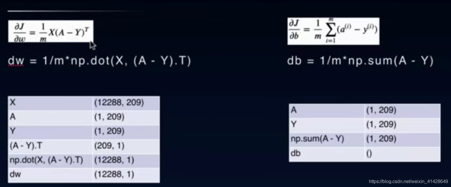
反向傳播的公式推導是比較難的，但是推導出來後用程式碼是比較好實現的，
上圖列出了矩陣維度的變化，唯一要注意的是最後運算出來的dw和db是跟前向傳播的w和b維度是一樣的。

# GRADED FUNCTION: propagate

def propagate(w, b, X, Y):
    """
    Implement the cost function and its gradient for the propagation explained above

    Arguments:
    w -- weights, a numpy array of size (num_px * num_px * 3, 1)
    b -- bias, a scalar
    X -- data of size (num_px * num_px * 3, number of examples)
    Y -- true "label" vector (containing 0 if non-cat, 1 if cat) of size (1, number of examples)

    Return:
    cost -- negative log-likelihood cost for logistic regression
    dw -- gradient of the loss with respect to w, thus same shape as w
    db -- gradient of the loss with respect to b, thus same shape as b
    
    Tips:
    - Write your code step by step for the propagation. np.log(), np.dot()
    """
    
    m = X.shape[1]
    
    # FORWARD PROPAGATION (FROM X TO COST)
    A = sigmoid(np.dot(w.T, X) + b)          
    cost = -1/m * np.sum(Y * np.log(A) + (1-Y) * np.log(1-A))
    
    # BACKWARD PROPAGATION (TO FIND GRAD)
    dw = 1/m * np.dot(X, (A-Y).T)
    db = 1/m * np.sum(A-Y)
    assert(dw.shape == w.shape)
    assert(db.dtype == float)
    cost = np.squeeze(cost)
    assert(cost.shape == ())
    
    grads = {"dw": dw,
             "db": db}
    
    return grads, cost

w, b, X, Y = np.array([[1],[2]]), 2, np.array([[1,2],[3,4]]), np.array([[1,0]])
grads, cost = propagate(w, b, X, Y)
print ("dw = " + str(grads["dw"]))
print ("db = " + str(grads["db"]))
print ("cost = " + str(cost))

Output:
dw = [[0.99993216]
[1.99980262]]
db = 0.49993523062470574
cost = 6.000064773192205

優化函數部分：

# GRADED FUNCTION: optimize

def optimize(w, b, X, Y, num_iterations, learning_rate, print_cost = False):
    """
    This function optimizes w and b by running a gradient descent algorithm
    
    Arguments:
    w -- weights, a numpy array of size (num_px * num_px * 3, 1)
    b -- bias, a scalar
    X -- data of shape (num_px * num_px * 3, number of examples)
    Y -- true "label" vector (containing 0 if non-cat, 1 if cat), of shape (1, number of examples)
    num_iterations -- number of iterations of the optimization loop
    learning_rate -- learning rate of the gradient descent update rule
    print_cost -- True to print the loss every 100 steps
    
    Returns:
    params -- dictionary containing the weights w and bias b
    grads -- dictionary containing the gradients of the weights and bias with respect to the cost function
    costs -- list of all the costs computed during the optimization, this will be used to plot the learning curve.
    
    Tips:
    You basically need to write down two steps and iterate through them:
        1) Calculate the cost and the gradient for the current parameters. Use propagate().
        2) Update the parameters using gradient descent rule for w and b.
    """
    
    costs = []
    
    for i in range(num_iterations):
        
        
        # Cost and gradient calculation (≈ 1-4 lines of code)  代價和梯度的計算
        grads, cost = propagate(w, b, X, Y)
        
        # Retrieve derivatives from grads
        dw = grads["dw"]
        db = grads["db"]
        
        # update rule (≈ 2 lines of code)  參數的更新
        w = w - learning_rate * dw    #學習率乘以梯度
        b = b - learning_rate * db
        
        # Record the costs
        if i % 100 == 0:
            costs.append(cost)
        
        # Print the cost every 100 training examples
        if print_cost and i % 100 == 0:
            print ("Cost after iteration %i: %f" %(i, cost))
    
    params = {"w": w,
              "b": b}
    
    grads = {"dw": dw,
             "db": db}
    
    return params, grads, costs

params, grads, costs = optimize(w, b, X, Y, num_iterations= 100, learning_rate = 0.009, print_cost = False)
print ("w = " + str(params["w"]))
print ("b = " + str(params["b"]))
print ("dw = " + str(grads["dw"]))
print ("db = " + str(grads["db"]))

Output:
w = [[0.1124579 ]
[0.23106775]]
b = 1.5593049248448891
dw = [[0.90158428]
[1.76250842]]
db = 0.4304620716786828

預測結果：

# GRADED FUNCTION: predict

def predict(w, b, X):
    '''
    Predict whether the label is 0 or 1 using learned logistic regression parameters (w, b)
    
    Arguments:
    w -- weights, a numpy array of size (num_px * num_px * 3, 1)
    b -- bias, a scalar
    X -- data of size (num_px * num_px * 3, number of examples)
    
    Returns:
    Y_prediction -- a numpy array (vector) containing all predictions (0/1) for the examples in X
    '''
    
    m = X.shape[1]
    Y_prediction = np.zeros((1,m))
    w = w.reshape(X.shape[0], 1)
    
    # Compute vector "A" predicting the probabilities of a cat being present in the picture
    A = sigmoid(np.dot(w.T,X) + b)

    for i in range(A.shape[1]):
        
        # Convert probabilities A[0,i] to actual predictions p[0,i]
        if A[0,i]<=0.5:         #當預測結果小於0.5的時候等於0
            Y_prediction[0,i] = 0
        else:
            Y_prediction[0,i] = 1
    
    assert(Y_prediction.shape == (1, m))
    
    return Y_prediction

print ("predictions = " + str(predict(w, b, X)))

Output:
predictions = [[1. 1.]]

程式碼函數的整合：

# GRADED FUNCTION: model

def model(X_train, Y_train, X_test, Y_test, num_iterations = 2000, learning_rate = 0.5, print_cost = False):
    """
    Builds the logistic regression model by calling the function you've implemented previously
    
    Arguments:
    X_train -- training set represented by a numpy array of shape (num_px * num_px * 3, m_train)
    Y_train -- training labels represented by a numpy array (vector) of shape (1, m_train)
    X_test -- test set represented by a numpy array of shape (num_px * num_px * 3, m_test)
    Y_test -- test labels represented by a numpy array (vector) of shape (1, m_test)
    num_iterations -- hyperparameter representing the number of iterations to optimize the parameters
    learning_rate -- hyperparameter representing the learning rate used in the update rule of optimize()
    print_cost -- Set to true to print the cost every 100 iterations
    
    Returns:
    d -- dictionary containing information about the model.
    """
   
    
    # initialize parameters with zeros (≈ 1 line of code)
    w, b = initialize_with_zeros(X_train.shape[0])

    # Gradient descent (≈ 1 line of code)
    parameters, grads, costs = optimize(w,b,X_train,Y_train,num_iterations,learning_rate,print_cost)
    
    # Retrieve parameters w and b from dictionary "parameters"
    w = parameters["w"]
    b = parameters["b"]
    
    # Predict test/train set examples (≈ 2 lines of code)
    Y_prediction_test = predict(w,b,X_test)
    Y_prediction_train = predict(w,b,X_train)

    # Print train/test Errors
    print("train accuracy: {} %".format(100 - np.mean(np.abs(Y_prediction_train - Y_train)) * 100))
    print("test accuracy: {} %".format(100 - np.mean(np.abs(Y_prediction_test - Y_test)) * 100))

    
    d = {"costs": costs,
         "Y_prediction_test": Y_prediction_test, 
         "Y_prediction_train" : Y_prediction_train, 
         "w" : w, 
         "b" : b,
         "learning_rate" : learning_rate,
         "num_iterations": num_iterations}
    
    return d

d = model(train_set_x, train_set_y, test_set_x, test_set_y, num_iterations = 2000, learning_rate = 0.005, print_cost = True)
#迭代數是2000，學習率是0.005

Output:
Cost after iteration 0: 0.693147
Cost after iteration 100: 0.584508
Cost after iteration 200: 0.466949
Cost after iteration 300: 0.376007
Cost after iteration 400: 0.331463
Cost after iteration 500: 0.303273
Cost after iteration 600: 0.279880
Cost after iteration 700: 0.260042
Cost after iteration 800: 0.242941
Cost after iteration 900: 0.228004
Cost after iteration 1000: 0.214820
Cost after iteration 1100: 0.203078
Cost after iteration 1200: 0.192544
Cost after iteration 1300: 0.183033
Cost after iteration 1400: 0.174399
Cost after iteration 1500: 0.166521
Cost after iteration 1600: 0.159305
Cost after iteration 1700: 0.152667
Cost after iteration 1800: 0.146542
Cost after iteration 1900: 0.140872
train accuracy: 99.04306220095694 %
test accuracy: 70.0 %
#輸出了訓練過程和結果

測試部分：

# Example of a picture that was wrongly classified.
index = 6
plt.imshow(test_set_x[:,index].reshape((num_px, num_px, 3)))
print ("y = " + str(test_set_y[0,index]) + ", you predicted that it is a \"" + classes[int(d["Y_prediction_test"][0,index])].decode("utf-8") +  "\" picture.")

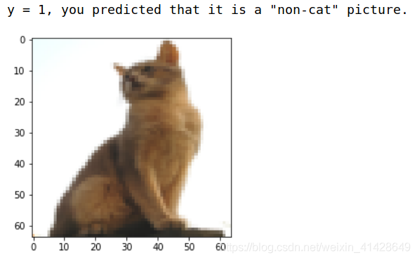
很明顯，上述這個結果就錯了。

# Plot learning curve (with costs)
costs = np.squeeze(d['costs'])
plt.plot(costs)
plt.ylabel('cost')
plt.xlabel('iterations (per hundreds)')
plt.title("Learning rate =" + str(d["learning_rate"]))
plt.show()

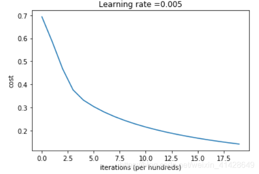
Interpretation: You can see the cost decreasing. It shows that the parameters are being learned. However, you see that you could train the model even more on the training set. Try to increase the number of iterations in the cell above and rerun the cells. You might see that the training set accuracy goes up, but the test set accuracy goes down. This is called overfitting.

進一步分析：

learning_rates = [0.01, 0.005, 0.001, 0.0005, 0.0001]
models = {}
for i in learning_rates:
    print ("learning rate is: " + str(i))
    models[str(i)] = model(train_set_x, train_set_y, test_set_x, test_set_y, num_iterations = 1500, learning_rate = i, print_cost = False)
    print ('\n' + "-------------------------------------------------------" + '\n')

for i in learning_rates:
    plt.plot(np.squeeze(models[str(i)]["costs"]), label= str(models[str(i)]["learning_rate"]))

plt.ylabel('cost')
plt.xlabel('iterations')

legend = plt.legend(loc='upper center', shadow=True)
frame = legend.get_frame()
frame.set_facecolor('0.90')
plt.show()

learning rate is: 0.01
train accuracy: 99.52153110047847 %
test accuracy: 68.0 %

---

learning rate is: 0.005
train accuracy: 97.60765550239235 %
test accuracy: 70.0 %

---

learning rate is: 0.001
train accuracy: 88.99521531100478 %
test accuracy: 64.0 %

---

learning rate is: 0.0005
train accuracy: 82.77511961722487 %
test accuracy: 56.0 %

---

learning rate is: 0.0001
train accuracy: 68.42105263157895 %
test accuracy: 36.0 %

---

不同的學習率在迭代次數的增加下，cost的變化過程
可以試着自己新增學習率檢視結果

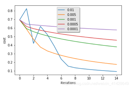
Interpretation:

Different learning rates give different costs and thus different predictions results.
If the learning rate is too large (0.01), the cost may oscillate up and down. It may even diverge (though in this example, using 0.01 still eventually ends up at a good value for the cost).
A lower cost doesn't mean a better model. You have to check if there is possibly overfitting. It happens when the training accuracy is a lot higher than the test accuracy.
In deep learning, we usually recommend that you:
    Choose the learning rate that better minimizes the cost function.
    If your model overfits, use other techniques to reduce overfitting. (We'll talk about this in later videos.)

最後一步就是利用我們訓練好的分類器來測試自己的圖片

## START CODE HERE ## (PUT YOUR IMAGE NAME) 
my_image = "cat_in_iran.jpg"   # change this to the name of your image file 
## END CODE HERE ##

# We preprocess the image to fit your algorithm.
fname = "images/" + my_image
image = np.array(ndimage.imread(fname, flatten=False))
my_image = scipy.misc.imresize(image, size=(num_px,num_px)).reshape((1, num_px*num_px*3)).T
my_predicted_image = predict(d["w"], d["b"], my_image)

plt.imshow(image)
print("y = " + str(np.squeeze(my_predicted_image)) + ", your algorithm predicts a \"" + classes[int(np.squeeze(my_predicted_image)),].decode("utf-8") +  "\" picture.")

然後我遇到了這個錯誤
檢查過後發現是缺少了一個pillow包，安裝即可