資料探勘中的12種距離度量原理及實現程式碼
2021-05-05 07:00:43
本文介紹了12種常用的距離度量原理、優缺點、應用場景,以及基於Numpy和Scipy的Python實現程式碼。
筆記工具:Notability
文章目錄
- 1. 個人筆記
- 2. 程式碼實現
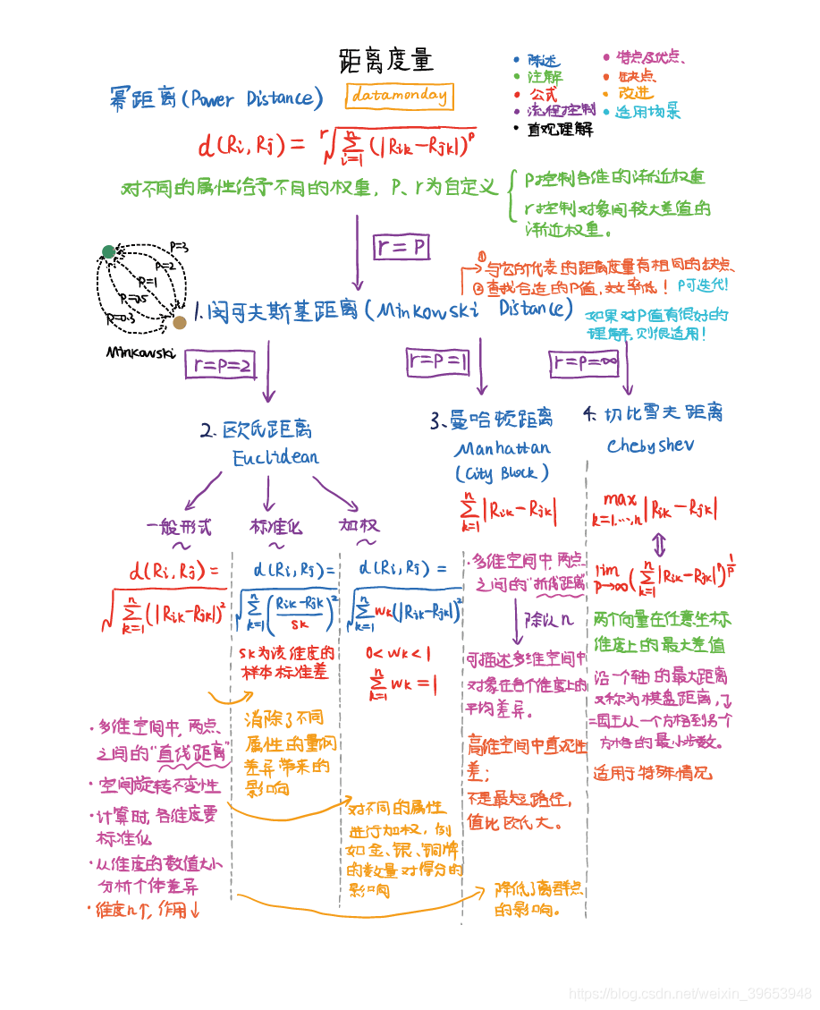
- 1)閔可夫斯基距離(Minkowski Distance)
- 2) 歐氏距離(Euclidean Distance)
- 3) 曼哈頓距離(Manhattan/City Block Distance)
- 4) 切比雪夫距離(Chebyshev Distance)
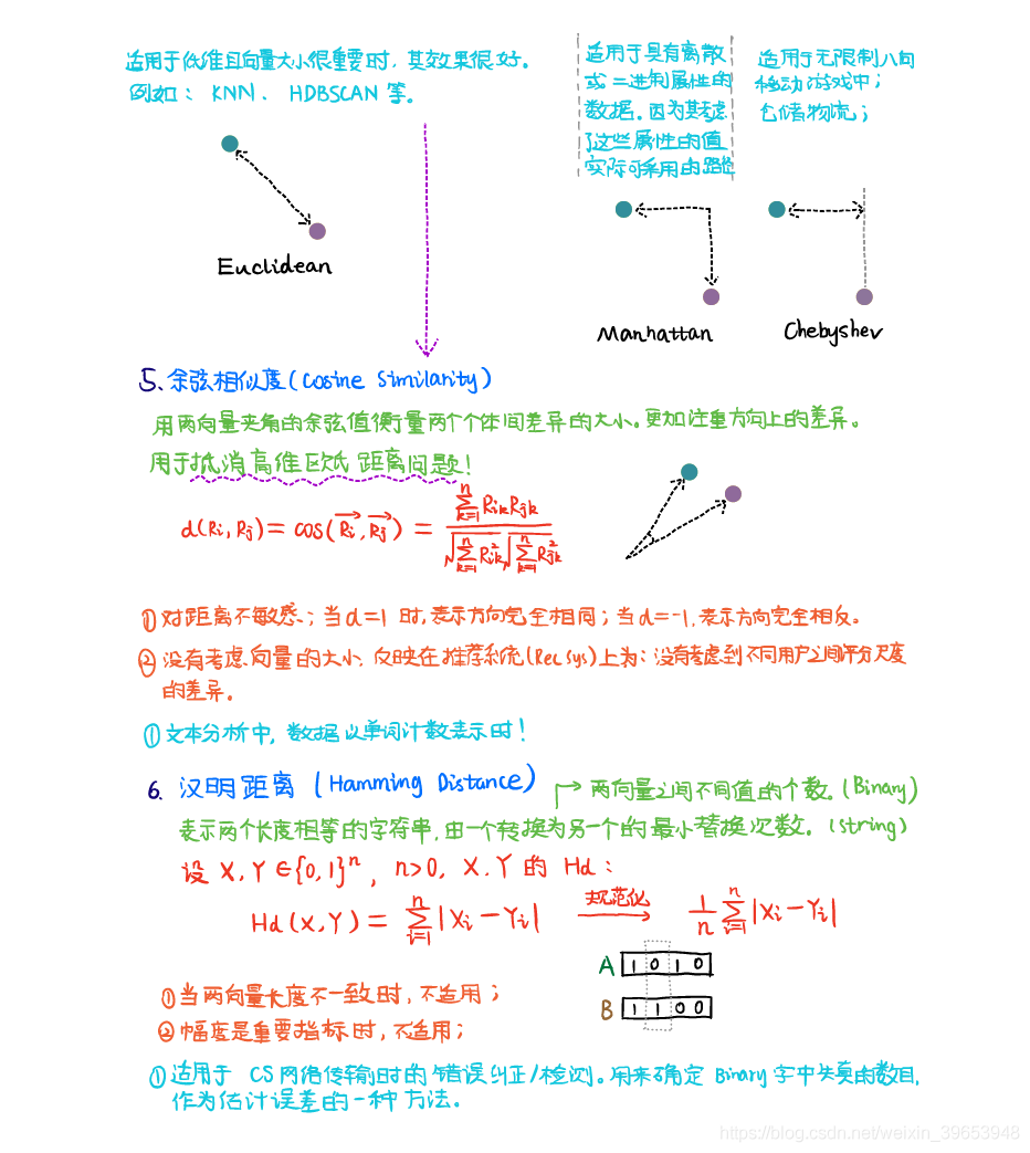
- 5) 餘弦相似度(Cosine Similarity)
- 6) 漢明距離(Hamming Distance)
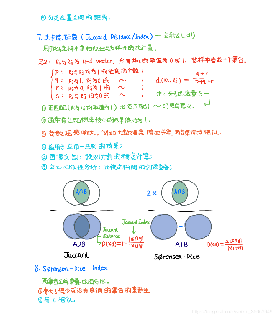
- 7) 傑卡德距離(Jaccard Distance)
- 8) S Φ rensen-Dice
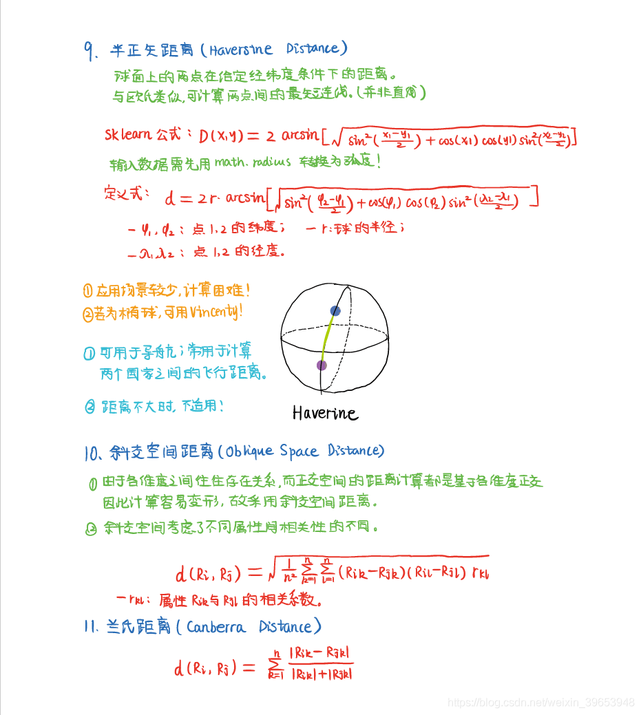
- 9) 半正矢距離(Haversine Distance)
- 10) 斜交空間距離(Oblique Space Distance)
- 11) 蘭氏距離(Canberra Distance)
- 12) 馬氏距離(Mahalanobis Distance)
1. 個人筆記
筆記工具:Notability
筆記獲取:
- 公眾號: datazero 回覆:DM 獲取下載地址。(主頁左側邊欄掃碼)
- Github:https://github.com/datamonday/BigDataAnalysis
2. 程式碼實現
匯入必要的包,並構造資料。
import numpy as np
from scipy.spatial.distance import pdist

x = np.random.random(5)
# array([0.75173729, 0.34763686, 0.71927609, 0.24151473, 0.22294162])

y = np.random.random(5)
# array([0.98036113, 0.45482745, 0.87472311, 0.92923963, 0.62922737])
1)閔可夫斯基距離(Minkowski Distance)
# p = 2 ——> 歐氏距離
pdist(xy, metric="minkowski", p=2)
2) 歐氏距離(Euclidean Distance)
# 根據公式求解
np.sqrt(np.sum(np.square(x - y) ) )

# 0.8520305805970781
# 根據scipy庫求解
xy = np.vstack([x, y])
pdist(xy, metric="euclidean")

# array([0.85203058])
3) 曼哈頓距離(Manhattan/City Block Distance)
np.sum(np.abs(x - y))

# 1.585272101374208
pdist(xy, metric="cityblock")

# array([1.5852721])
4) 切比雪夫距離(Chebyshev Distance)
np.max(np.abs(x - y))

# 0.6877248997688814
pdist(xy, metric="chebyshev")

# array([0.6877249])
5) 餘弦相似度(Cosine Similarity)
np.dot(x, y) / ( np.linalg.norm(x) * np.linalg.norm(y) )

# 0.9232011981703329
1 - pdist(xy, metric="cosine")

# array([0.9232012])
6) 漢明距離(Hamming Distance)
np.mean( x != y )

# 1.0
pdist(xy, metric="hamming")

# array([1.])
7) 傑卡德距離(Jaccard Distance)
molecular = np.double( (x != y).sum() )
denominator = np.double(np.bitwise_or( x != 0, y != 0).sum() )

molecular / denominator

# 1.0
pdist(xy, metric="jaccard")

# array([1.])
8) S Φ rensen-Dice
pdist(xy, metric="dice")

# array([0.])
9) 半正矢距離(Haversine Distance)
"""
計算Ezeiza機場(阿根廷布宜諾斯艾利斯)和戴高樂機場(法國巴黎)之間的距離。
"""

from sklearn.metrics.pairwise import haversine_distances
from math import radians

bsas = [-34.83333, -58.5166646]
paris = [49.0083899664, 2.53844117956]

bsas_in_radians = [radians(_) for _ in bsas]
paris_in_radians = [radians(_) for _ in paris]

result = haversine_distances([bsas_in_radians, paris_in_radians])
# multiply by Earth radius to get kilometers
result * 6371000/1000
輸出:
array([[    0.        , 11099.54035582],
       [11099.54035582,     0.        ]])
10) 斜交空間距離(Oblique Space Distance)
11) 蘭氏距離(Canberra Distance)
np.sum( np.true_divide( np.abs(x - y), np.abs(x) + np.abs(y) ) )

# 1.4272762731136441
pdist(xy, metric="canberra")

 # array([1.42727627])
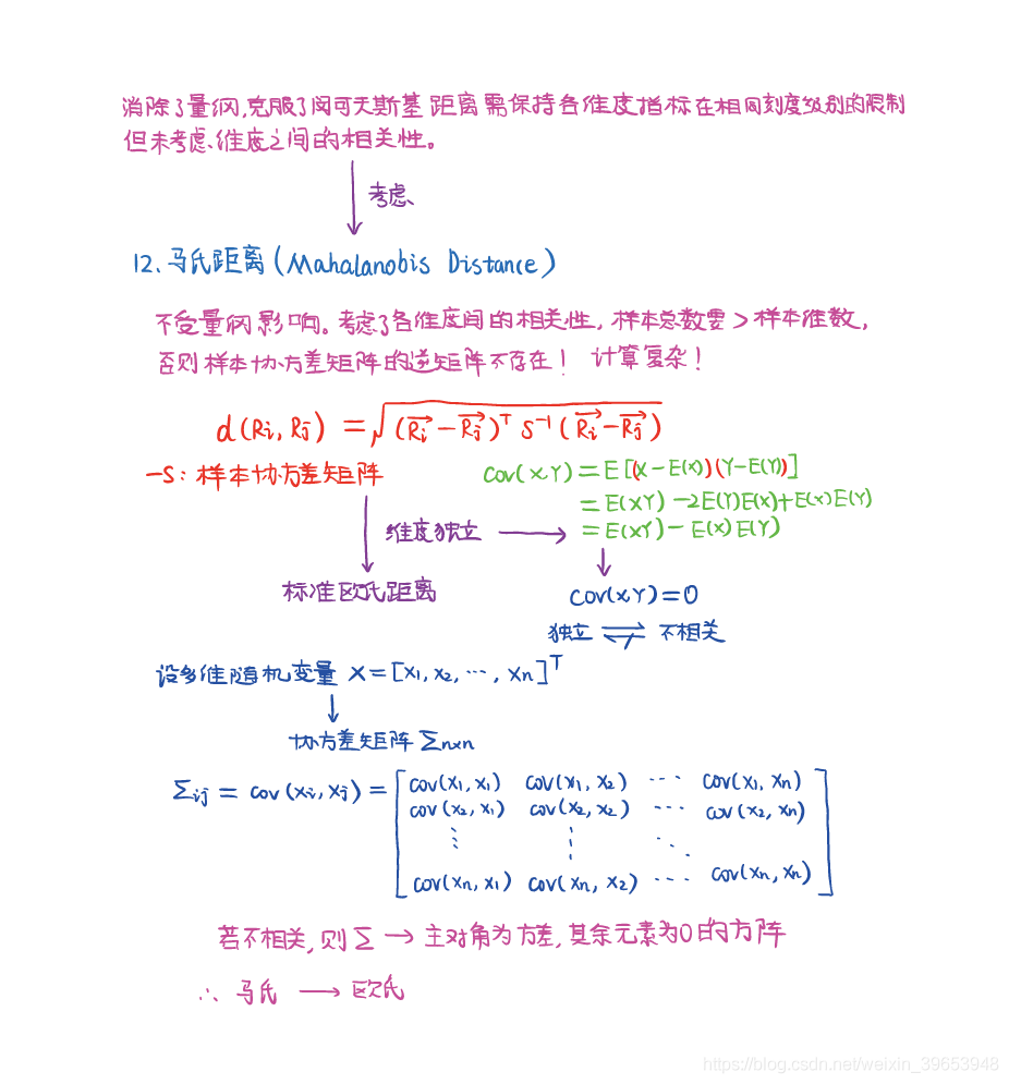
12) 馬氏距離(Mahalanobis Distance)
-
馬氏距離要求樣本個數>維數,此處重新生成樣本集:10個樣本,2個屬性;
-
馬氏距離計算兩兩樣本之間的距離,故結果包含: C 10 2 = 45 C^{2}_{10} = 45 C102=45 個距離分量。
data = np.random.random([10, 2])
data # (10, 2)
array([[0.16057991, 0.03173777],
       [0.04984203, 0.63608966],
       [0.0965663 , 0.54125706],
       [0.14562222, 0.50749436],
       [0.12384608, 0.66895134],
       [0.38362246, 0.96750912],
       [0.66204458, 0.34832719],
       [0.62169272, 0.76812896],
       [0.55320254, 0.59736334],
       [0.53135375, 0.97430267]])
# 求解個維度之間協方差矩陣
S = np.cov(data.T)
# 計算協方差矩陣的逆矩陣
ST = np.linalg.inv(S)
ST
array([[18.39262731, -4.22549979],
       [-4.22549979, 13.68987876]])
n = data.shape[0]
d1 = []

for i in range(0, n):
    for j in range(i + 1, n):
        delta = data[i] - data[j]
        d = np.sqrt( np.dot( np.dot(delta, ST), delta.T) )
        d1.append(d)

print(len(d1))
d1
45
[2.4064983868149823,
 1.9761163000756812,
 1.778448926503528,
 2.404430793536302,
 3.3375019493285927,
 2.1576814382238196,
 2.9094250412104405,
 2.3104822379986585,
 3.426008151540264,
 0.4480137866843753,
 0.7065459737678685,
 0.30815685501580464,
 1.618002146140689,
 3.0847744520164553,
 2.3696411013587313,
 2.2012364723722557,
 2.1104688855720037,
 0.2717792884385083,
 0.4554926318973598,
 1.7230353296945067,
 2.7042335514201556,
 2.183968292942155,
 1.9135693479813816,
 2.1102154148029593,
 0.6287347650129346,
 1.735958615801837,
 2.438573435905017,
 2.012440681515558,
 1.6900976084983395,
 2.048918972209157,
 1.3438862451280977,
 2.862373485815439,
 2.067854534269353,
 1.928870122984677,
 1.8108503250774675,
 2.851523901145603,
 1.409891022070067,
 1.7131869461579778,
 0.6273442013634126,
 1.608018006961265,
 1.1384164544766362,
 2.5238527095532692,
 0.6218088758251554,
 0.94309743685501,
 1.422491582300723]
pdist(data, metric="mahalanobis")
array([2.40649839, 1.9761163 , 1.77844893, 2.40443079, 3.33750195,
       2.15768144, 2.90942504, 2.31048224, 3.42600815, 0.44801379,
       0.70654597, 0.30815686, 1.61800215, 3.08477445, 2.3696411 ,
       2.20123647, 2.11046889, 0.27177929, 0.45549263, 1.72303533,
       2.70423355, 2.18396829, 1.91356935, 2.11021541, 0.62873477,
       1.73595862, 2.43857344, 2.01244068, 1.69009761, 2.04891897,
       1.34388625, 2.86237349, 2.06785453, 1.92887012, 1.81085033,
       2.8515239 , 1.40989102, 1.71318695, 0.6273442 , 1.60801801,
       1.13841645, 2.52385271, 0.62180888, 0.94309744, 1.42249158])
Reference:
- 《巨量資料分析與挖掘》 ch5:聚類演演算法
- 資料科學中常見的9種距離度量方法,內含歐氏距離、切比雪夫距離等
- 9 Distance Measures in Data Science