在寫論文的時候瞭解到有fasttext這種文字分類方法，也看了很多別人的部落格，但感覺使用這種方法的人並不是很多，或者使用的版本有些舊。本文會介紹下Windows下最新的fasttext版本以及如何進行文字分類

文章目錄

fasttext簡介
Windows下安裝
版本
- 新版特色
- 主要函數及用法
文字分類
小節

以下是本篇文章正文內容，下面案例可供參考

fasttext簡介

fasttext是2016年facebook開源的一款高效詞表示和文字分類工具。它是一個淺層的神經網路模型，類似於word2vec的CBOW，主要用途就是兩個——詞向量化和文字分類。

官網: https://fasttext.cc/docs/en/python-module.html.

Windows下安裝

程式碼如下（範例）：

pip install fasttext

版本

2019年6月25官網釋出了Windows下的最新版本，這個版本將原來的官方版fastText和非官方版fasttext合併,現在最新版本fasttext在github repository和 pypi.org都可以找到。

新版特色

保留了官方API和頂層函數（例如train_unsupervised和train_supervised）以及返回的numpy物件。從非正式API中刪除了cbow，skipgram和supervised函數。並且將非官方API中的好主意帶到了官方API中。特別是，我們喜歡WordVectorModel這類很python的方法。

主要函數及用法

如果是文字分類用到的函數就是 train_supervised

import fasttext

model = fasttext.train_supervised('data.train.txt')

這裡data.train.txt是一個文字檔案，每行包含一個訓練語句以及標籤。預設情況下，我們假設標籤是帶有字串__label__字首的string.

該函數主要引數如下：

 input             # training file path (required)
    lr                # learning rate [0.1]
    dim               # size of word vectors [100]
    ws                # size of the context window [5]
    epoch             # number of epochs [5]
    minCount          # minimal number of word occurences [1]
    minCountLabel     # minimal number of label occurences [1]
    minn              # min length of char ngram [0]
    maxn              # max length of char ngram [0]
    neg               # number of negatives sampled [5]
    wordNgrams        # max length of word ngram [1]
    loss              # loss function {ns, hs, softmax, ova} [softmax]
    bucket            # number of buckets [2000000]
    thread            # number of threads [number of cpus]
    lrUpdateRate      # change the rate of updates for the learning rate [100]
    t                 # sampling threshold [0.0001]
    label             # label prefix ['__label__']
    verbose           # verbose [2]
    pretrainedVectors # pretrained word vectors (.vec file) for supervised learning []
    #可以用訓練好的詞向量

文字分類

資料集

這裡用攜程酒店評論資料https://www.kesci.com/home/dataset/5e620482b8dfce002d803622
共有7766條其中正向5322條，負向2444條。

import pandas as pd 
import numpy as np
from sklearn  import metrics
from sklearn import model_selection
from sklearn.naive_bayes import BernoulliNB
import jieba
from xgboost import plot_importance,plot_tree
import xgboost as xgb
import fasttext
import time

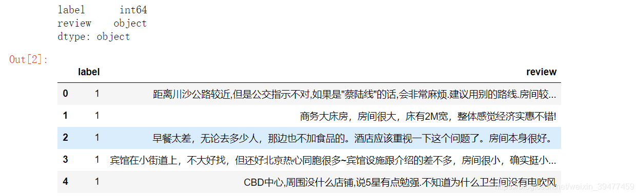
df = pd.read_csv('D:word data/ChnSentiCorp_htl_all.csv',encoding='utf-8')
df = df.dropna()
print(df.dtypes)
df.head()

前五條資料

資料處理

分詞和去除停用詞

def filter_stopwords(txt):
    sent = jieba.lcut(txt)
    words = []
    for word in sent:
        if(word in stopwords):
            continue
        else:
            words.append(word)
    return ' '.join(words)

def get_custom_stopwords(stop_words_file):
    with open(stop_words_file,encoding="utf8") as f:
        stopwords = f.read()
    stopwords_list = stopwords.split('\n')
    custom_stopwords_list = [i for i in stopwords_list]
    return custom_stopwords_list

stop_words_file = 'D:/data/stoplist.txt'
stopwords = get_custom_stopwords(stop_words_file)

文字格式處理

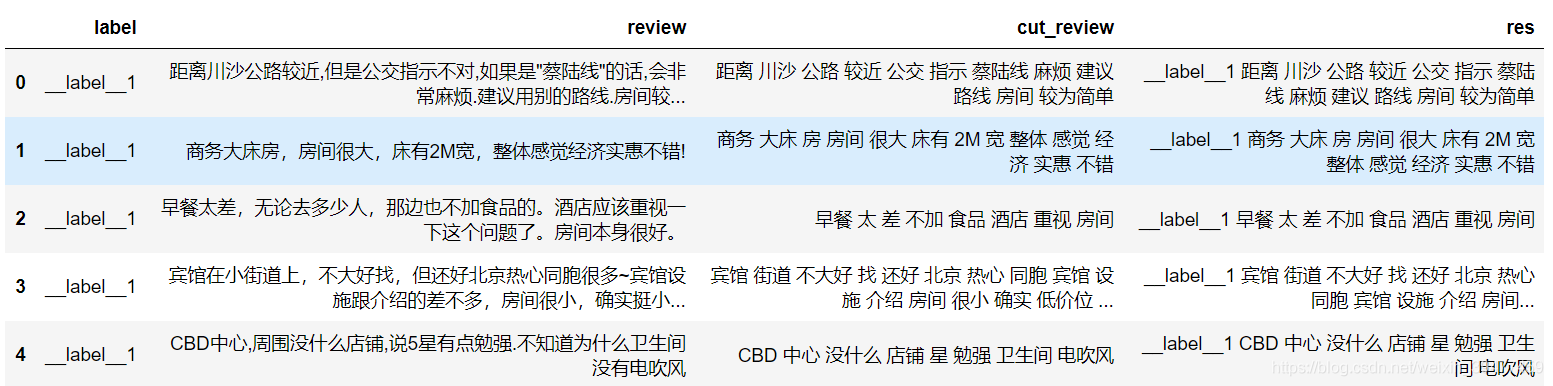
df['cut_review'] = df.review.apply(filter_stopwords)
df['label'] = '__label__'+ df['label'] #fasttext需要將分類標籤添上'__label__'字首
#且要求每行輸出如下中間用分隔符分開，而','分隔符是不行的
df['res'] = df['label'] + ' ' + df['cut_review']

處理後資料

劃分資料集並儲存為txt檔案

由於train_supervised中input引數只接受檔案路徑，劃分資料集為訓練集和測試集後儲存為text檔案

sentences = df['res']
sentences_train,sentences_test = train_test_split(sentences,test_size = 0.3)
sentences_train = sentences_train.values.tolist()
sentences_test = sentences_test.values.tolist()

def writeData(sentences,fileName):
    print("writing data to fasttext format...")
    out=open(fileName,'w',encoding='utf-8')
    for sentence in sentences:
        out.write(sentence+"\n")
    print("done!")

fileName = 'D:word data/ChnSentiCorp_htl_train.txt'
writeData(sentences_train,fileName)
fileName = 'D:word data/ChnSentiCorp_htl_test.txt'
writeData(sentences_test,fileName)

二分類

ts = time.time()
model = fasttext.train_supervised('D:word data/ChnSentiCorp_htl_train.txt')
time.time() - ts
# 0.2246713638305664

#模型評估
def print_results(N, p, r):
    print("N\t" + str(N))
    print("P@{}\t{:.3f}".format(1, p))
    print("R@{}\t{:.3f}".format(1, r))

print_results(*model.test('D:word data/ChnSentiCorp_htl_test.txt'))


# N	2330
# P@1	0.861 precsion 這可能是正樣本比例偏高導致的
# R@1	0.861 recall

調參

#考慮word ngram 並改損失函數為負取樣的損失函數
ts = time.time()
model = fasttext.train_supervised('D:word data/ChnSentiCorp_htl_train.txt',wordNgrams = 2，loss = 'ns')
time.time() - ts
# 0.2246713638305664

#模型評估
def print_results(N, p, r):
    print("N\t" + str(N))
    print("P@{}\t{:.3f}".format(1, p))
    print("R@{}\t{:.3f}".format(1, r))

print_results(*model.test('D:word data/ChnSentiCorp_htl_test.txt'))
# N	2330
# P@1	0.856
# R@1	0.856
#效果並沒有提高

和樸素貝葉斯比較

#匯入資料並處理
df = pd.read_csv('D:word data/ChnSentiCorp_htl_all.csv',encoding='utf-8')
df = df.dropna()
df['cut_review'] = df.review.apply(filter_stopwords)
X = df['cut_review']
y = df.label
X_train, X_test, y_train, y_test = train_test_split(X, y, test_size=0.3, random_state=22)

#詞向量化 只考慮每個單詞出現的頻率；然後構成一個特徵矩陣，每一行表示一個訓練文#本的詞頻統計結果
from sklearn.feature_extraction.text import CountVectorizer
vect = CountVectorizer(max_df = 0.8, 
                       min_df = 3, 
                       token_pattern=u'(?u)\\b[^\\d\\W]\\w+\\b', 
                       stop_words=frozenset(stopwords))

from sklearn.naive_bayes import MultinomialNB
nb = MultinomialNB()

X_train_vect = vect.fit_transform(X_train)
nb.fit(X_train_vect, y_train)
train_score = nb.score(X_train_vect, y_train)
print(train_score)
# 0.895363811976819

#模型評估
pred = nb.predict(X_test_vect)
y_test
X_test_vect = vect.transform(X_test)
metrics.precision_score(y_test,nb.predict(X_test_vect)),metrics.recall_score(y_test,pred)
# (0.8984088127294981, 0.9157829070492826)
# 樸素貝葉斯效果還是好一些的

小節

本文僅僅簡單介紹了fasttext的使用，可能資料集比較小，又是簡單的二分類任務，fasttext優勢並沒有展現出來，之後會用更大的訓練集和多分類任務進行測試。

Windows下fasttext文字分類